3. Tools

The main menu toolbar features the tools dropdown menu. In EE-UQ, tools are applications designed to generate inputs for specific workflow applications or are tools providing useful functionality for our users. For instance, the ShakerMaker tool helps to simulate ground motions from earthquakes, providing essential input data for further structural analysis and engineering assessments.

3.1. Domain Reduction Method Analysis

Domain Reduction Method analysis tool in EE-UQ is user interface through which users can create a model in OpenSees and use the implemented DRM loading in OpenSees to perform a high fidelity analysis of a structure subjected to earthquake ground motions. The DRM analysis tool is designed to simplify the process of creating a model using parallel processing and doing the analysis using OpenSeesMP through TACC facilities. The tool is designed to be user-friendly and to provide a seamless experience for users to perform a DRM analysis.

3.1.1. Domain Reduction Method

The Domain Reduction Method (DRM) helps to simplify complex earthquake simulations, making it easier and faster to compute how buildings and structures react to earthquakes. Here’s a simple breakdown:

3.1.1.1. Why is this needed?

In areas near a fault (the break in the Earth’s crust where earthquakes happen), the ground moves in a unique way. To study how earthquakes affect large regions, we need to run computer models of these ground motions. However, these models are often very slow and take up a lot of computing power. That’s where the DRM comes in—it helps reduce the amount of computing needed while still getting accurate results.

3.1.1.2. What is DRM?

DRM is a method that divides the problem into two smaller parts, which makes the whole process faster and more manageable. It was first developed by researchers named Bielak and Yoshimura in 2003.

3.1.1.3. How does it work?

1. Step 1: Solve a Big Picture Problem (Background Problem) First, you solve a “big picture” problem. This means you model a large area that includes both the earthquake waves and the area around the structure (like a building) you are interested in. In this step, you focus on how the earthquake waves move through the ground, not the specific details of what happens to the building.

2. Step 2: Focus on the Area Near the Structure (Local Problem) After you have a good idea of how the earthquake waves move, you can zoom in and focus just on the building or structure. The earthquake waves from Step 1 are applied to the building, and you can study how the building reacts to these waves. This step allows you to include detailed effects, like cracks or bending that might happen to the structure.

figure fig-ShakerMaker_DRM shows two stages of the DRM process.

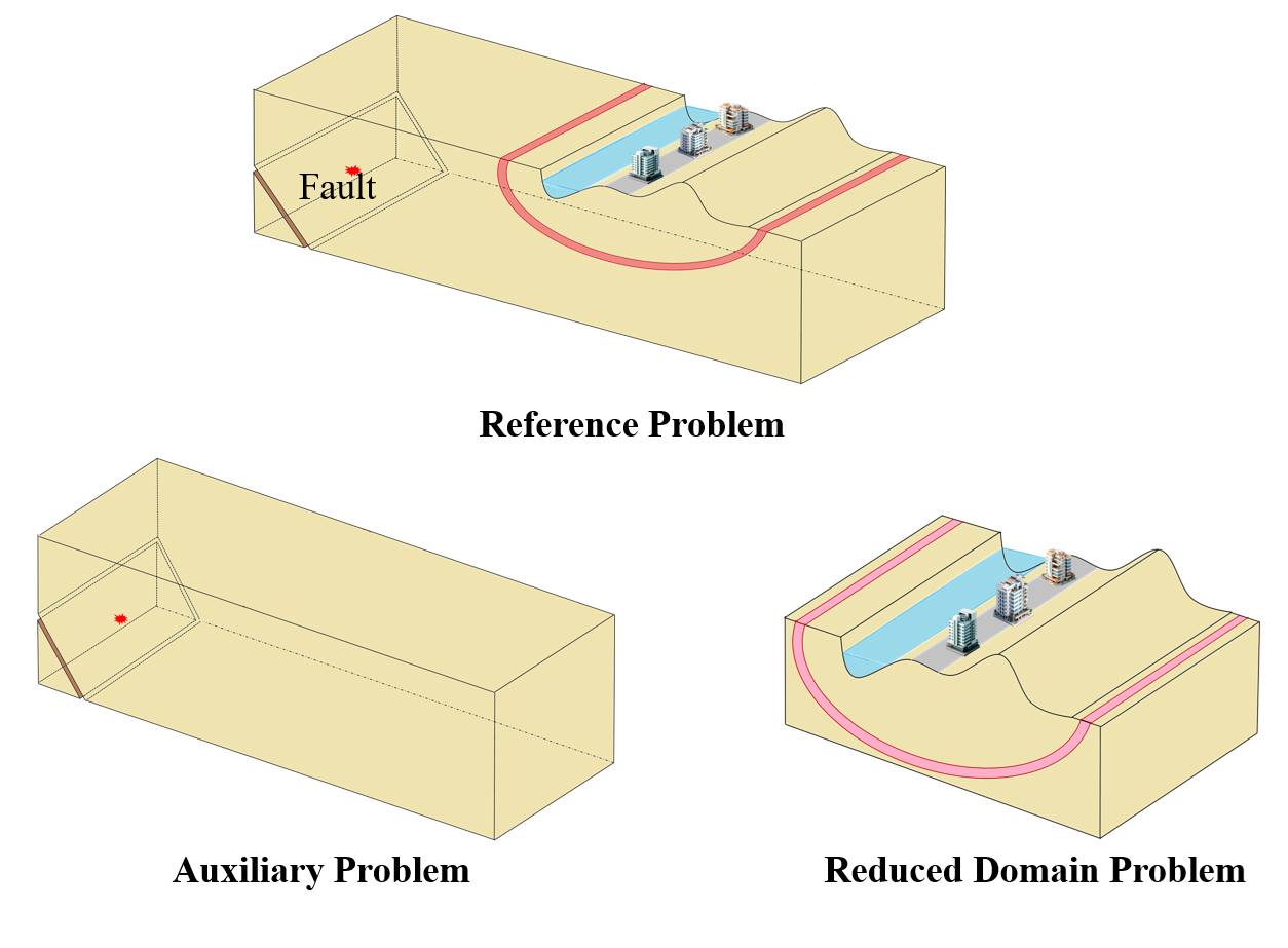
Fig. 3.1.1.3.1 Two stages of the DRM.

3.1.1.4. Why is this method useful?

This two-step method saves a lot of time. Instead of having to model both the entire earthquake region and the building in one big, slow calculation, DRM breaks it down. First, you solve the larger, simpler problem (earthquake waves in a big region), and then you use that information to do a more detailed and focused analysis on just the building.

Despite its advantages, the DRM has seen limited use due to challenges in handling large, complex datasets, which require specialized tools for creation. ShakerMaker addresses these issues by offering a straightforward solution for generating DRM-compatible motions and an accessible format for working with extensive datasets, making it easier for researchers and practitioners to leverage this powerful method in their analyses. There is functionality in OpenSees which accept a DRM load in hdf5 format. The DRM loading should be in a special format which some software like ShakerMaker can generate. The DRM loading is applied to the model in OpenSeesMP and the analysis is performed using TACC facilities.

3.1.2. Domain Reduction Method Analysis user interface

The DRM analysis tool user interface is consists of the six sections:

• Soil Properties: This section allows the user to define soil geometry and properties.

• DRM Layer: This section allows the user to define the number of DRM layers and the properties input DRM load.

• Absorbing Layers: This section allows the user to define the number of absorbing layers and the properties of the absorbing layers.

• Partitiones: This section allows the user to define the number of partitions for each of soil, DRM and absorbing layers.

• Analysis Information: This section allows the user to define the analysis parameters for the OpenSees model.

• Job Information: This section allows the user to submit the job to TACC facilities and get the results back.

3.1.2.1. Soil Properties

Right now, the DRM analysis tool only supports a single soil layer with cube geometry. The user can define the geometry by inputting the Width in X, Y and Z directions in meters and the number of elements in X, Y and Z directions. For the properties of the single layer of soil, the user can input the density, shear wave velocity and Poisson’s ratio.

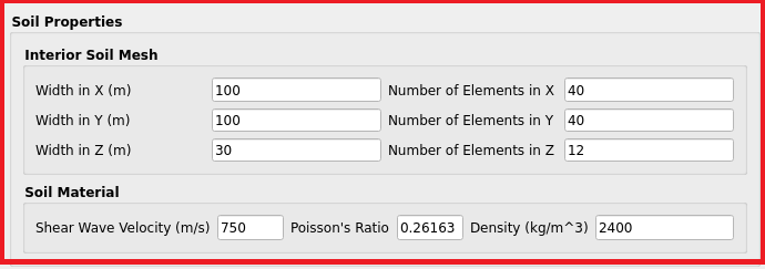
Fig. 3.1.2.1.1 DRM Analysis Tool Soil Properties Section.

3.1.2.2. DRM Layer

The DRM layer section allows the user to define the number of DRM layers and the properties of the DRM load. The DRM Software dropdown allows the user to select the software used to generate the DRM load. The only change that this dropdown does is to change the default values of the properties of the DRM load. Right now, ShakerMaker and Custom are the only options in the dropdown. The Propertises of the DRM Load is aligned with the parameters in H5DRM pattern: H5DRM Documentation in OpenSees. The user can input the properties of the DRM load in the textboxes provided. The properties are:

• Number of Layers: The number of layers around the Soil layer.

• Coordinate Transformation check: The checkbox to enable the coordinate transformation. if checked, the DRM load used the coordinate transformation provided by the user otherwise the default coordinate in the DRM load is used.

• Load Factor: The load factor applied to the DRM load.

• Coordinate Scale: The scale factor applied to the DRM points coordinates to match the point coordinates in the model.

• Tolerance: The tolerance used in the DRM pattern to match the points in the DRM load to the points in the model.

• T11, T12, T13, T21, T22, T23, T31, T32, T33: The transformation matrix for coordinate transformation if the coordinate transformation is checked.

• DRM File Location: The location of the DRM load file. The user can access the file in their local machine or in the DesignSafe workspace.

• DRM File Path: The path to the DRM load file in either the local machine or the DesignSafe workspace.

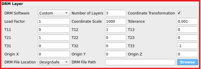
Fig. 3.1.2.2.1 DRM Analysis Tool DRM Layer Section.

Notes: - Right now for submitting job to TACC, the DRM load file should be in the DesignSafe workspace other wise users will need to upload the DRM load file to the DesignSafe workspace and provide the path to the file in the DRM File Path textbox. - If user want to browse the DRM load file in the DesignSafe workspace, they can click on the Browse button and a window will pop up showing the files in the DesignSafe workspace. User may need to login to DesignSafe first by passing username and password in another window that will pop up when the Browse button is clicked. Users then can use backward and forward buttons to navigate through the files and folders and select button to select the file. The path to the file will be automatically filled in the DRM File Path textbox.

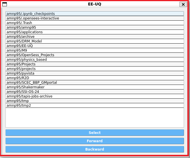
Fig. 3.1.2.2.2 Browse DRM Load File in DesignSafe Workspace.

3.1.2.3. Absorbing Layers

The Absorbing Layers section allows the user to define the type and number of absorbing layers. The user can select the type of absorbing layers from the dropdown. The options are PML elements, ASDA elements, and Normal Elements with Rayleigh Damping. In the case of Normal Elements with Rayleigh Damping, the user can input the damping ratio in the provided text box. However, for PML elements and ASDA elements, the text box is disabled, as the damping ratio is not required.

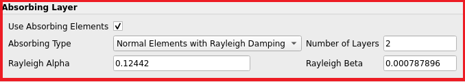
Fig. 3.1.2.3.1 DRM Analysis Tool Absorbing Layers Section.

3.1.2.4. Partitiones

The Partitiones section allows the user to define the number of partitions for each of soil, DRM and absorbing layers. The user can select the partitioning method from the dropdown. Right now, the only option in the dropdown is KD-Tree. The user can input the number of partitions in the text For each of the soil, DRM and absorbing layers, at least one partition is required so the minimum cores required for the analysis is 3.

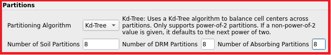
Fig. 3.1.2.4.1 DRM Analysis Tool Partitiones Section.

Notes: - KD-Tree needs power of 2 number of partitions. If the user inputs a number that is not a power of 2, the tool will automatically round it up to the next power of 2.

3.1.2.5. Analysis Information

The Analysis Information section allows the user to define the analysis parameters for the OpenSees model and create the model. The user can input the analysis parameters in the textboxes provided. The parameters are:

• Time Step (s): The time step for the analysis.

• Final Time (s): The final time for the analysis.

• Recording Time Step (s): The time step for recording the results.

• Output Directory: The directory where the output files will be saved. The default directory is the local EE-UQ workspace in the subdirectory DRM_Model.

The user can click on the Create Model button to create the model in OpenSees. By clicking on the button, the tool will create Model in the subdirectory of Mesh from the choosen output directory and shows the mesh int Visualization window on the right side of the tool under different tabs. The user can click on the tabs to see the mesh of the soil, DRM and absorbing layers. The user can also click on the Download Model button to download the model in the zip format.

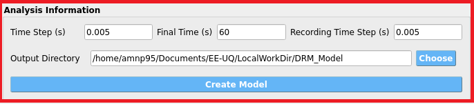
Fig. 3.1.2.5.1 DRM Analysis Tool Analysis Information Section.

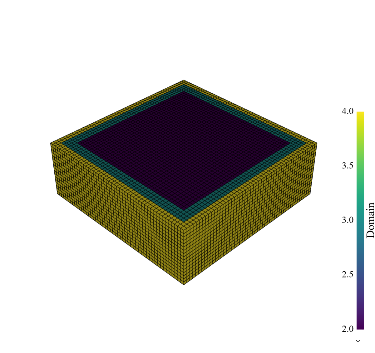
Fig. 3.1.2.5.2 Domain mesh visualization.

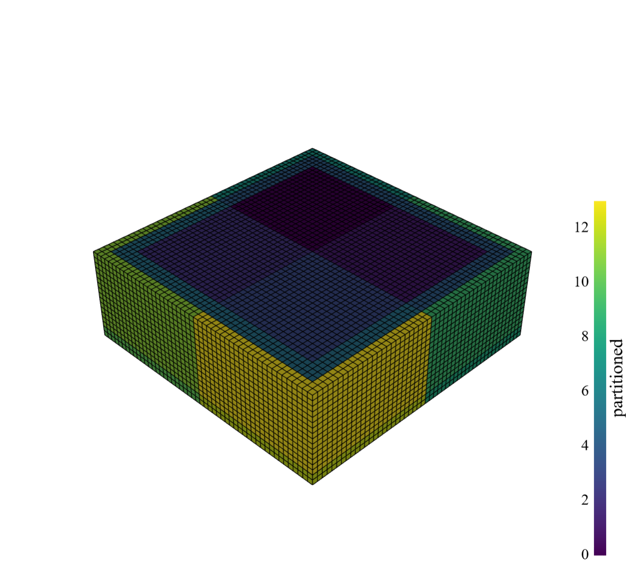
Fig. 3.1.2.5.3 Partitioned mesh visualization.

3.1.2.6. Job Information

The Job Information section allows the user to submit the job to TACC facilities and get the results back. The user can input the job parameters in the textboxes provided. The parameters are:

• System: The system to run the job on. The options are available systems in TACC.

• Allocation: The allocation of the user in TACC.

• Maximum Run Time: The maximum run time for the job.

• Job UUID: The unique identifier for the job.

By pressing the Submit Job button, the tool will create a model first and then submit the job to TACC facilities. The UUID of the job will be shown in the Job UUID textbox. The user can click on the Get Results button to get the results of the job. The results will be downloaded in the output directory provided in the Analysis Information section in the subdirectory Results. The result of these analysis will be the accelration, velocity and displacement time history of the model at center of the soil layer in X, Y and Z directions in a json format. User can use this json files to continue the analysis in the EEUQ by putting the time histories on different structures and running the analysis.

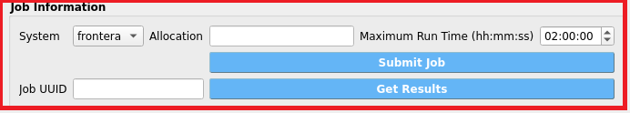
Fig. 3.1.2.6.1 DRM Analysis Tool Job Information Section.

3.2. ShakerMaker Tool

ShakerMaker is a Python library designed for generating and analyzing seismic wave motions. Its core functionality is built upon the FK method, which is implemented in Fortran. This allows ShakerMaker to leverage the high-performance capabilities of Fortran while providing a user-friendly interface through Python. ShakerMaker is designed to assist both earthquake engineers and seismologists by providing an easy-to-use tool for generating and exploring ground motions using the frequency-wavenumber (FK) method on 1-D crustal models. This innovative tool allows users to create realistic, physics-based waveforms for various earthquake scenarios, which can then be analyzed using the Domain Reduction Method (DRM).

The DRM facilitates the simulation of how soil and structures respond to ground motions during earthquakes by connecting large regional earthquake simulations with smaller local soil-structure models without losing critical details. This method significantly improves the accuracy of ground-motion simulations.

ShakerMaker tool is a graphical user interface within the EEUQ framework that allows users to create ShakerMaker models easily. This tool simplifies the process of modeling seismic events by providing a visual platform for users to define and manipulate various parameters related to faults, crustal layers and stations. Users can load available fault models and select the type of station they wish to use based on the crustal model. The ShakerMaker tool then generates the necessary input files for the ShakerMaker engine and runs the simulation, providing users with the resulting ground motions for further analysis.

3.2.1. Coordinate system in ShakerMaker

ShakerMaker defines it’s coordinate system with x positive towards the north, y positive towards the east and z positive downwards. Strike is defined clockwise from the north, dip is measured from the horizontal, and rake increases in the down-dip direction.

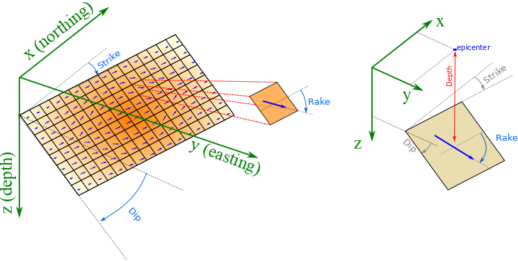
Fig. 3.2.1.1 ShakerMaker coordinate system.

3.2.2. ShakerMaker tool workflow

The ShakerMaker tool in EEUQ follows a simple workflow to generate ground motions. The interface is divided into five main sections:

1. Analysis Information: This section allows users to define the analysis parameters.

2. Source Information: This section provides options to define the fault model.

3. Material Layers: This section allows users to define the crustal model.

4. Station Information: This section provides options to define the station model.

5. Job and Visualization: This section allows users to view the fualt model and submit the job for processing.

3.2.2.1. Analysis Information

The Analysis Information section allows users to define the analysis parameters. The parammeters which can be defined are:

• dt: Time step for the simulation in seconds.

• nfft : Number of points in the frequency domain. It needs to be a power of 2. Not e that the more number of points, the more accurate the simulation will be but it will also take more time.

• dk: Wavelength increment in the frequency domain. The default value is 0.2 which is a good value for most simulations but can be changed if needed.

• tmin: Minimum time for the simulation in seconds

• tmax: Maximum time for the simulation in seconds. The simulation will run from tmin to tmax. Note that the duration of should be greater than nfft*dt.

• dh: Horizontal spacing critera for creating green’s functions database for DRM load. This parameters is only used when your are creating a DRM load. The default value is 40 meters.

• dv_rec: Vertical spacing critera between station points in a DRM station for creating green’s functions database for DRM load. This parameters is only used when your are creating a DRM load. The default value is 200 meters.

• dv_src: Vertical spacing critera between source points in a fault for creating green’s functions database for DRM load. This parameters is only used when your are creating a DRM load. The default value is 5 meters.

• tmp Directory: Temporary directory where the simulation files will be stored. This directory should have enough space to store the simulation files. The default value is the ShakerMaker folder in the EEUQ working directory.

Note: The default values are good for most simulations. Only parameters which are needed to be changed may be tmax based on the durtion and distance of the stations from the fault.

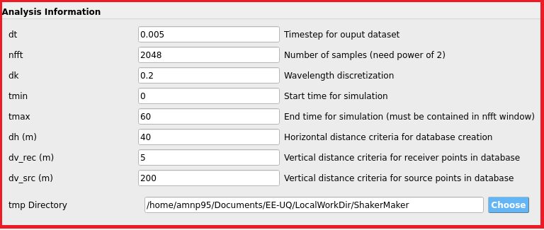
Fig. 3.2.2.1.1 Analysis box interface.

3.2.2.2. Source Information

The Source Information section provides options to define the fault model. The base idea is that user can just load the fault model from the available fault models in the ShakerMaker tool.

for the fault model user can pick the fault considered fault model from the drop down menu. The drop down menu is in the Load From Database section. The laoding section has 5 drop down menus. the first one is for the country of the fault model, the second one is for the name of the fault model (which shows the region) and the other three are Magnitude, Type and Realization which are specific to a specific fault. By pressing the the Load Database button the fault information automatically gets loaded in the Source Information and fault files will be downloaded in the tmp Directory user defined in the Analysis Information under the subfolder of fault.

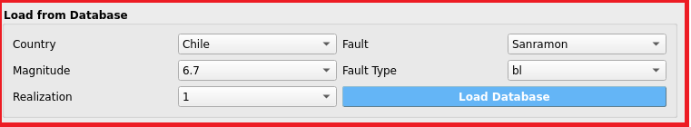
Fig. 3.2.2.2.1 Load fault interface.

user can also define their own fault model by providing the fault latitude, longitude and the realted json fault files. The fault files should be in special format which will be explained in the next release of the ShakerMaker tool.

3.2.2.3. Material Layers

The Material Layers section allows users to define the crustal model. The crustal model is defined by the number of layers and the properties of each layer. for definig the layers a table is provided where user can add rows and define the properties of each layer. properties of each layer are:

• Layer Name: Name of the layer. This is just for the user to identify the layer.

• Thickness: Thickness of the layer in km.

• Vp: P wave velocity in km/s.

• Vs: S wave velocity in km/s.

• Density: Density of the layer in g/cm^3.

• Qp: Q factor for P wave.

• Qs: Q factor for S wave.

Each crustal layer at least has one infite layer which is the half space and is shown by the last row with a tickness of 0.

Also there is a load from File section which allows user to load the crustal model from a json file. the json file should be array of objects where each object is a layer with the keys (name, thickness, vp, vs, density, qp, qs).

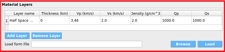
Fig. 3.2.2.3.1 Material Layers interface.

3.2.2.4. Station Information

The Station Information section provides options to define the station model. The stations can be single stations or a DRM station. which each one can be choosen from the drop down menu.

single station

For the single station user can define the station latitude, longitude and the depth of the station. The depth is the distance from the surface of the earth to the station in km. Users can add multiple stations by pressing the Add Station button. The stations can be removed by pressing the Remove Station button. Also, user can open a map to select the station location by pressing the Open Map button and find the station latitude, longitude and using the google map.

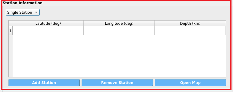
Fig. 3.2.2.4.1 Single Station interface.

DRM station

DRM Station is available by choosing the DRM box from the menu. The DRM station is a set of stations around a center on a surface in terms of cube. so the parameters for the DRM station are:

• Latitude: Latitude of the center of the cube.

• Longitude: Longitude of the center of the cube.

• Width X: Width of the cube in the North-South direction in m.

• Width Y: Width of the cube in the East-West direction in m.

• Depth: Depth of the cube in m.

• Mesh Size (x): Mesh size in the North-South direction in m to discretize the cube.

• Mesh Size (y): Mesh size in the East-West direction in m to discretize the cube.

• Mesh Size (z): Mesh size in the vertical direction in m to discretize the cube.

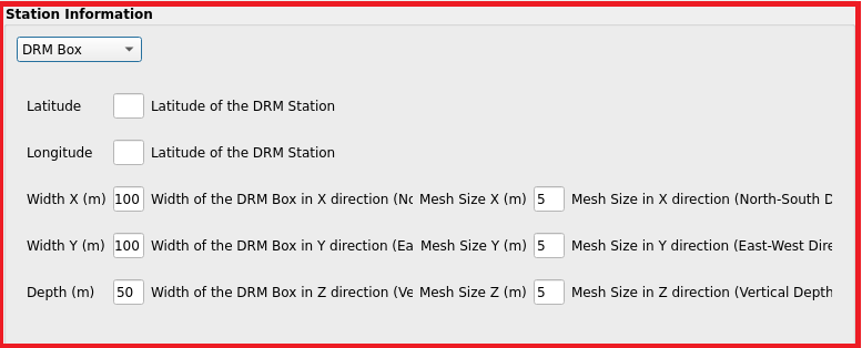
Fig. 3.2.2.4.2 DRM Station interface.

3.2.2.5. Job and Visualization

The Job and Visualization section allows users to sumit a job and run shakermaker model in TACC facilities and visualize the fault. This part contains of two serated box. The job box and the visualization box. .. _fig-ShakerMaker_Job:

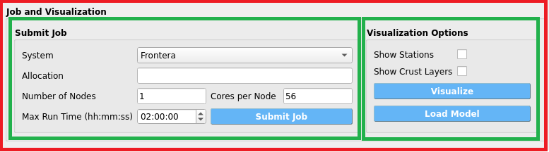
Fig. 3.2.2.5.1 Job interface.

Job

The job part get information about the job and submit the job to the TACC facilities. The parameters are:

• System: The system which the job will be submitted. The default value is frontera.

• Allocation: The allocation which the job will be charged. Users should provide their own allocation.

• Number of Nodes: Number of nodes which the job will be run on. The default value is 1.

• Cores per Node: Number of cores per node. The default value is 56 for frontera.

• Maximum run time: Maximum run time for the job in hours. The default value is 2 hours.

Note : if you are using DRM station it is recommended to use at least 200 cores (Nodes multiply by cores per node) for the job with a mximum run time of at least 10 hours.

Visualization

The visualization part allows users to visualize the fault model. The visulaization will be shown in the right side of the ShakerMaker panel. The visualization consits of two tabs. One that shows the plane of the fault in the plot tab and other one that shows the fault on the map. In the visualization box there are two other check boxes, one for showing the stations on the map and the other one for showing the crustal model on the plot tab. By pressing the Visualize button a python code will be run and the fault will be shown in the plot tab and the map tab after a while. Both plots are interactive and user can zoom in and out and move the plot.

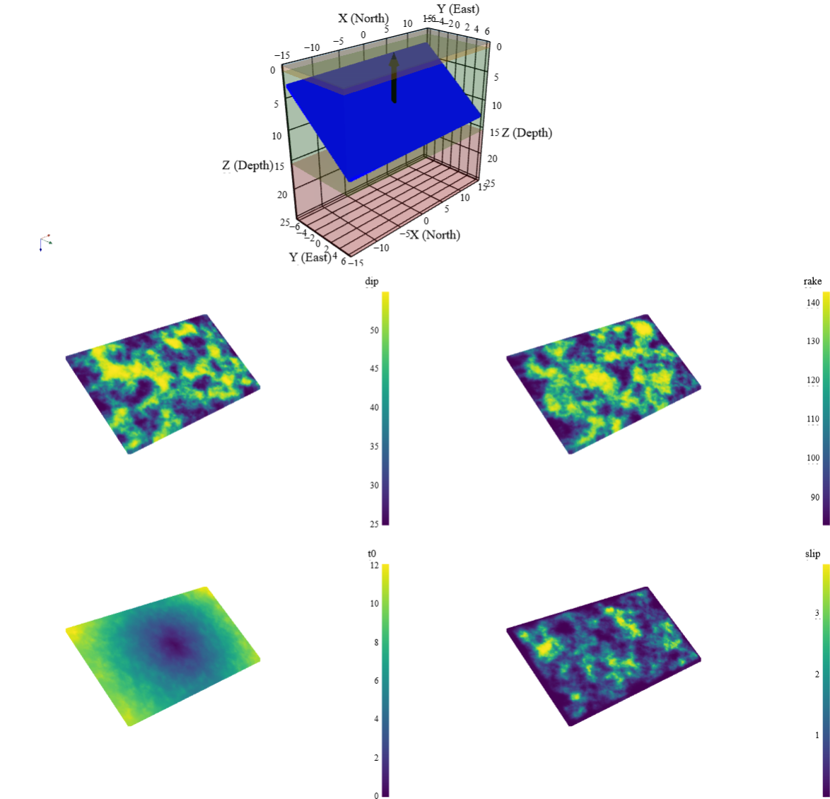
Fig. 3.2.2.5.2 Fault visualization.

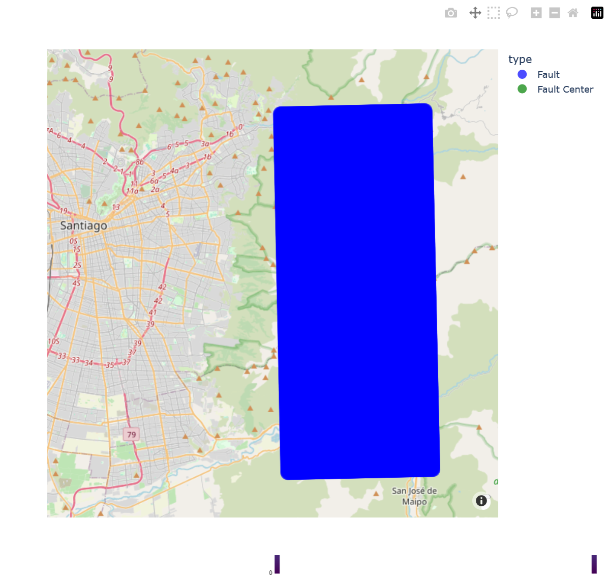
Fig. 3.2.2.5.3 Fault visualization on the map.

Also in the visulaization box there is a Load Model button. By pressing this button a browsing window will be opened and user can load whole model from a json file. In the applications folder, under the subdirectory tools/Shakermaker/Examples, there are two example files:

• DRM_Sanramon.json

• Single_Sanramon.json

Here is an example of the json file for the loading ShakerMaker parameters with a DRM station:

{
    "dt": 0.005,
    "nfft": 2048,
    "dk": 0.2,
    "tmin": 0,
    "tmax": 60,
    "dh": 40.0,
    "dv_rec": 5.0,
    "dv_src": 200,
    "layers": [
        {"Layer Name": "Layer1", "Thickness": 0.20, "Vp": 1.32, "Vs": 0.75, "Density": 2.4, "Qp": 1000, "Qs": 1000},
        {"Layer Name": "Layer2", "Thickness": 0.80, "Vp": 2.75, "Vs": 1.57, "Density": 2.5, "Qp": 1000, "Qs": 1000},
        {"Layer Name": "Layer3", "Thickness": 14.5, "Vp": 5.50, "Vs": 3.14, "Density": 2.5, "Qp": 1000, "Qs": 1000},
        {"Layer Name": "Half Space Layer", "Thickness": 0, "Vp": 7.00, "Vs": 4.00, "Density": 2.67, "Qp": 1000, "Qs": 1000}
    ],
    "station_type": "DRM",
    "station_info": {
        "Latitude": -33.40657,
        "Longitude": -70.50653,
        "Width X": 105,
        "Width Y": 105,
        "Depth": 30,
        "Mesh Size X": 2.5,
        "Mesh Size Y": 2.5,
        "Mesh Size Z": 2.5
    },
    "fault_type": "Database",
    "fault_info": {
        "Country": "Chile",
        "Fault": "Sanramon",
        "Magnitude": "6.7",
        "Fault Type": "bl",
        "Realization": "3"
    },
    "System": "Frontera",
    "Queue": "development",
    "Number of Nodes": 40,
    "Cores per Node": 50,
    "Max Run Time": "02:00:00"
}


.. [Abell 2022] José A. Abell, Jorge G.F. Crempien, Matías Recabarren, ShakerMaker: A framework that simplifies the simulation of seismic ground-motions, SoftwareX, Volume 17, 2022, 100911, ISSN 2352-7110, https://doi.org/10.1016/j.softx.2021.100911. (https://www.sciencedirect.com/science/article/pii/S235271102100159X)

3.3. OpenSees@DesignSafe Tool

This tool allows users to submit OpenSees, OpenSeesSP, OpenSeesMP, and OpenSeesPy scripts to ** TACC ** to be run on some of the most powerful HPC computers in the world. The only requirement for users is that they have a ** DesignSafe ** account and an allocation at TACC, which can be obtained by submitting a ticket to DesignSafe requesting HPC access to ** Frontera ** and ** Stampede3 **.

As shown in the figure below, the user provides a memorable job name, the input script to run, the application to use, and its version. When the user selects the Run at DesignSafe button, additional inputs are requested, such as the number of nodes, the number of processors per node, the maximum runtime in minutes, and the allocation to use.

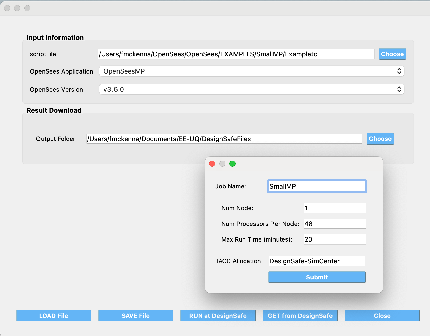
Fig. 3.3.1 OpenSees@DesignSafe Tool

After pressing the Submit button, the tool will zip the folder containing the script and, using Tapis, create a folder in your DesignSafe DataDepot account. The zipped file will be sent to this folder, and a simcenter-opensees job will be submitted to run with this folder and the selected application. Once the job is complete, the contents of the folder, now containing output files, will be zipped again and stored in DesignSafe for you.

To check the status of the submitted job and download the final folder, click the Get from DesignSafe button. A table will appear, showing the status of all submitted jobs. By right-clicking on any job in the table, a menu will appear with the option to Retrieve Data. If this option is selected, the zipped folder will be retrieved, unzipped, and the contents will be placed in the currently specified Output Folder.

Caution

Gotcha’s to running OpenSees scripts at DesignSafe

Given how this application runs, or any DesignSafe OpenSees offering, the script you run can only reference files in it’s current directory or directories below the current. Nor can the script save files outside of these locations.

Note

** 1. Which version of OpenSeesPy is run? **

The version run depends on your setup on the TACC HPC machine. All the tool does is run python3 in your working environment. What is run as a consequence is the first python3 application found on your path.

** 2. Why run OpenSees Jobs utilzing this application at DesignSafe? **

1. DesignSafe is providing access to some of the fastest HPC computers in the world, you can run for example OpenSeesMP jobs that utilize thousands of processors.

2. You can be running multiple jobs at the same time, though here is a limit to how many you can have runing at once!

3. The resulting folder containing your scripts is stored at DesignSafe. You can get that data. assuming you gave them a memorable job name, for jobs that ran today, yesterday, last week, last month, last year, …

** 3. Why this tool and not submit through DesignSafe Workspace OpenSees offerings? **

It’s simply the quickest way of getting the files to DesignSafe and submitting the job!