1.1. Random field
Gaussian processes have a long history in the statistics community.
They have been particularly well developed in the image signal processing community under the name random field,
and in the geostatistics community under the name of kriging
, which is a generic name used by geostatisticians for a family of generalized least-squares regression algorithms
in recognition of the pioneering work of a mining engineer Danie Krige [Kri51]
All kriging estimators are but variants of the basic linear regression estimator [Goo97].
For instance, a simple kriging estimator can be defined as
(1.1.1)\[Z^*({u_\alpha}) = \phi_0 + \boldsymbol{\phi}^T\boldsymbol{Z}(\boldsymbol{u})\]
in which \(\phi_0\) and \(\boldsymbol{\phi}\) are combining coefficients;
\(\boldsymbol{Z}(\boldsymbol{u})\) is the measured expected values at location \(\boldsymbol{u}\).
If \(\boldsymbol{Z}(\boldsymbol{u})\) is second order stationary
(i.e., invariant and known expected value exists, noted as \(\boldsymbol{\mu}\)),
the observed values at location \(\boldsymbol{u}\) could be expressed as
(1.1.2)\[\boldsymbol{Z}(\boldsymbol{u}) = \boldsymbol{\mu}+\boldsymbol{\epsilon}(\boldsymbol{u})\]
where \(\boldsymbol{\epsilon}(\boldsymbol{u})\) is the error vector with zero mean;
\(\boldsymbol{\mu}\) is the invariant and known mean value of this random field.
Hence the unobserved value at location \({u}_\alpha\) is
(1.1.3)\[{Z}({u}_\alpha) = {\mu}+{\epsilon}({u}_\alpha)\]
Simple kriging estimator should be unbiased:
(1.1.4)\[E[Z^*({u_\alpha})-{Z}({u}_\alpha)] = E[\phi_0
+ \boldsymbol{\phi}^T\boldsymbol{Z}(\boldsymbol{u})-{\mu}-{\epsilon}({u}_\alpha)]
=\phi_0+\boldsymbol{\phi}^T\boldsymbol{u}-\mu=0\]
This yields
(1.1.5)\[\phi_0=\mu - \boldsymbol{\phi}^T\boldsymbol{u}\]
Plug (1.1.5) into (1.1.1) so that the estimator becomes
(1.1.6)\[Z^*({u_\alpha}) = \mu+ \boldsymbol{\phi}^T ( \boldsymbol{Z}(\boldsymbol{u})-\boldsymbol{\mu} )
=\mu+\boldsymbol{\phi}^T\boldsymbol{\epsilon}(\boldsymbol{u})\]
Therefore the variance of the predicted values is
(1.1.7)\[\begin{split}\rm{Var}\{ Z^*({u_\alpha}) - Z({u_\alpha})\}
&=E[\mu+\boldsymbol{\phi}^T\boldsymbol{\epsilon}(\boldsymbol{u})-{\mu}-{\epsilon}({u}_\alpha)]^2 \\
&=E[\boldsymbol{\phi}^T\boldsymbol{\epsilon}(\boldsymbol{u})-{\epsilon}({u}_\alpha)]^2 \\
&=\rm{Var}\{\boldsymbol{\phi}^T\boldsymbol{\epsilon}(\boldsymbol{u}) \}
+\rm{Var}\{ {\epsilon}({u}_\alpha) \}-2\rm{COV}\{\boldsymbol{\phi}^T\boldsymbol{\epsilon}(\boldsymbol{u}),{\epsilon}({u}_\alpha) \} \\
&=\boldsymbol{\phi}^T\Sigma_{\boldsymbol{u},\boldsymbol{u}}\boldsymbol{\phi} + \rm{Var}\{\boldsymbol{Z}(\boldsymbol{u})\} -2\boldsymbol{\phi}^T \Sigma_{\boldsymbol{u},\alpha} \\\end{split}\]
To optimize \(\rm{Var}\{ Z^*({u_\alpha}) - Z({u_\alpha})\}\),
let its partial derivatives with respect to the vector of coefficients \(\boldsymbol{\phi}\) equate to zero
(1.1.8)\[\frac{\partial \left( \boldsymbol{\phi}^T\Sigma_{\boldsymbol{u},\boldsymbol{u}}\boldsymbol{\phi}
+ \rm{Var}\{\boldsymbol{Z}(\boldsymbol{u})\} -2\boldsymbol{\phi}^T \Sigma_{\boldsymbol{u},\alpha} \right)}{\partial \boldsymbol{\phi}}
=2\Sigma_{\boldsymbol{u},\boldsymbol{u}}\boldsymbol{\phi}-2\Sigma_{\boldsymbol{u},\alpha}=0\]
Hence
(1.1.9)\[\boldsymbol{\phi}=\Sigma_{\boldsymbol{u},\boldsymbol{u}}^{-1}\Sigma_{\boldsymbol{u},\alpha}\]
Plug ref{eq:phi} into ref{eq:estimatorSk_new} to obtained the simple kriging predictor
(1.1.10)\[Z^*({u_\alpha}) =
\mu+{\Sigma_{\boldsymbol{u},\alpha}}^T\Sigma_{\boldsymbol{u},\boldsymbol{u}}^{-1}
[\boldsymbol{Z}(\boldsymbol{u})-\boldsymbol{\mu}]\]
and the simple kriging variance is obtained as
(1.1.11)\[\begin{split}\rm{Var}\{ Z^*({u_\alpha}) - Z({u_\alpha})\}
&=\boldsymbol{\phi}^T\Sigma_{\boldsymbol{u},\boldsymbol{u}}\boldsymbol{\phi} + \rm{Var}\{\boldsymbol{Z}(\boldsymbol{u})\} -2\boldsymbol{\phi}^T \Sigma_{\boldsymbol{u},\alpha} \\
&=\boldsymbol{\phi}^T \Sigma_{\boldsymbol{u},\alpha} + \rm{Var}\{\boldsymbol{Z}(\boldsymbol{u})\} -2\boldsymbol{\phi}^T \Sigma_{\boldsymbol{u},\alpha}\\
&=\rm{Var}\{\boldsymbol{Z}(\boldsymbol{u})\}-\Sigma_{\boldsymbol{u},\alpha}^T
\Sigma_{\boldsymbol{u},\boldsymbol{u}}^{-1}
\Sigma_{\boldsymbol{u},\alpha}\end{split}\]
1.2. Neural Network
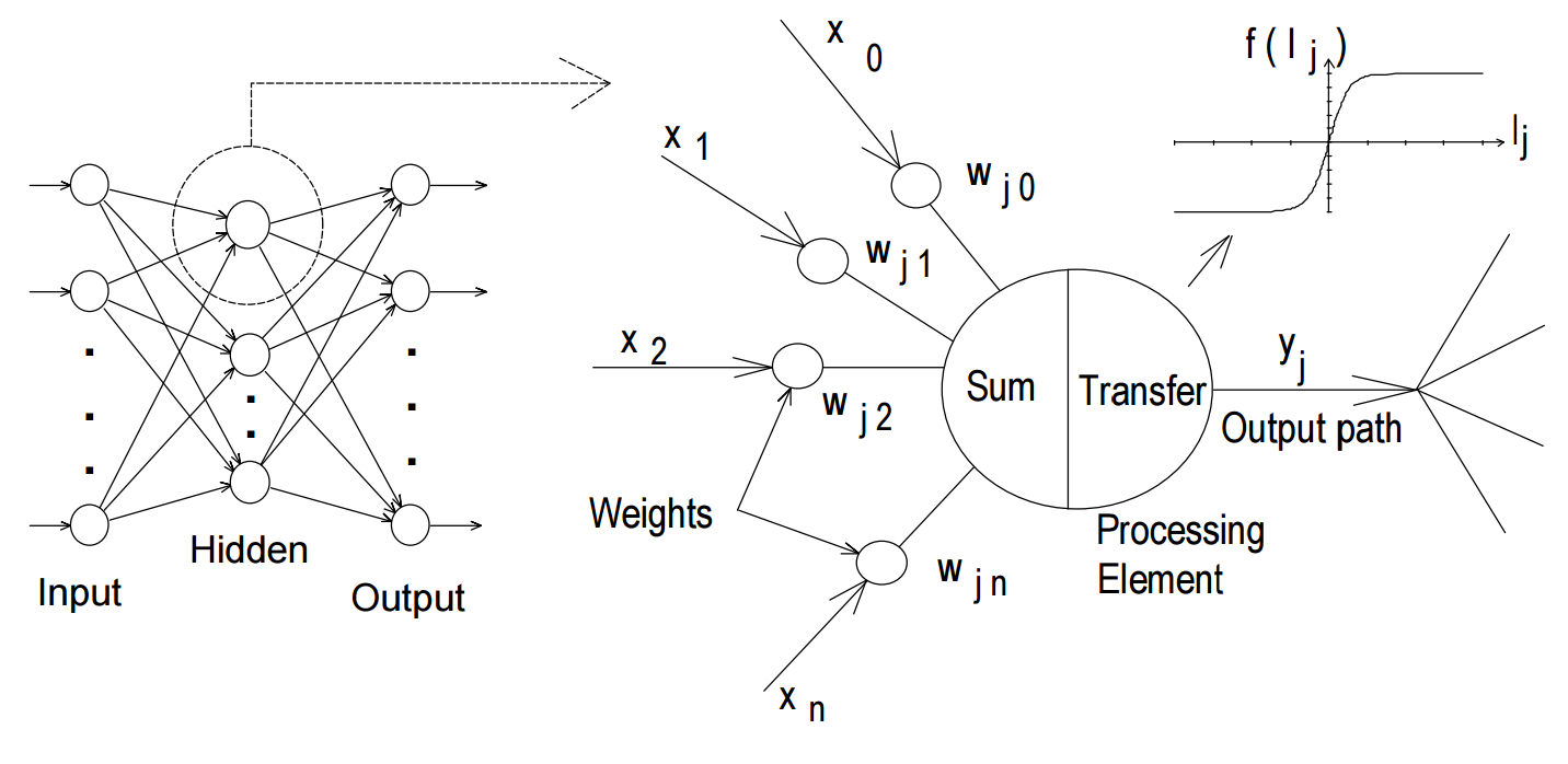
Artificial neural networks (ANNs) are a form of artificial intelligence which attempt to mimic the behavior of the human brain and nervous system. Many researchers have described the structure and operation of ANNs
(e.g. [HechtNielsenR90]; [Zur92]; [Fau94]). A typical structure of ANNs consists of a number of nodes (processing elements), that are usually arranged in layers: an input layer,
an output layer and one or more hidden layers (Fig. 1.2.1).
The input from each node in the previous layer (\(x_i\)) is multiplied by an adjustable connection weight (\(w_{ji}\)). At each node, the weighted input signals are summed and a threshold value (\(\theta_j\)) is added. This combined input
(\(I_j\)) is then passed through a non-linear transfer function (f(.)) to produce the output of the PE (\(y_i\)).
The output of one PE provides the input to the nodes in the next layer. This process is summarized in (1.2.1) and (1.2.2) and illustrated in Fig. 1.2.1.
(1.2.1)\[I_j=\sum w_{ji} x_i + \theta_j\]
(1.2.2)\[y_j = f(I_j)\]
The ANN modelling philosophy is similar to a number of conventional statistical models in the sense that both are attempting to capture the relationship between a historical set of model inputs and corresponding outputs. ANNs learn from data examples presented to them and use these data to adjust their weights in an attempt to capture the relationship between the model input variables and the corresponding outputs. Consequently, ANNs do not need any prior knowledge about the nature of the relationship between the input/output variables,
which is one of the benefits that ANNs have compared with most empirical and statistical methods.
ANNs have been applied in a great deal of research for a variety of purposes including medicine and biology ([MBN12];
[JS11]); pattern recognition and image analysis ([Bis95]; [YPL+00]; [Ami08]);
geotechnical engineering ([SJM08]);
decision making and control ([JR98]; [LB98]; [YAkyure07]; [ZGP10]);
and stock market predictions ([Dec10]) despite the disadvantages such as the black box nature and the
empirical nature of model development ([Tu96]).
ANNs are also widely used in spatial analysis and predictions of geotechnical and other engineering problems.
[SSA08] used ANN to evaluate the spatial variability of rock depth in an extended region.
[PM13] develop a scheme to generate prediction map for geostatistical data using ANN. When integrated with GIS geographic information system (GIS), ANN is a very powerful tool to make spatial analysis.
For example, [LRMW03] integrated with ANN to predict the regional landslide susceptibility. More works relating to ANN-GIS can be found
in [GGG99] [YAkyure07] [VLTSzatmari08], etc.
Spatial predictions with geostatistic tools (such as kriging methods) usually need a prescribed spatial correlation structure,
which should be inferred from measured data.
This is impossible when the size of the database is small.
One advantage of ANNs is that such a prescribed correlation structure is not needed.
Geostatistic tools, however, are still a good and widely used method for they are able to yield relatively precise and
spatially smooth predictions. Efforts to combine ANNs with traditional geostatistic tools have been made and can be found
in literature [RD94], [DKC+98] and [LHZ09].
| [Ami08] | J Amini. Optimum learning rate in back-propagation neural network for classification of satellite images (IRS-1D). Scientia Iranica, 15(6):558–567, 2008. |
| [Bis95] | Christopher M Bishop. Neural networks for pattern recognition. Oxford University Press, 1995. |
| [Dec10] | Porntip Dechpichai. Nonlinear neural network for conditional mean and variance forecasts. PhD thesis, University of Wollongong, New Zealand, 9 2010. |
| [DKC+98] | V Demyanov, M Kanevsky, S Chernov, E Savelieva, and V Timonin. Neural network residual kriging application for climatic data. Journal of Geographic Information and Decision Analysis, 2(2):215–232, 1998. |
| [Fau94] | L. Fausett. Fundamentals of neural networks: architectures, algorithms, and applications. Prentice-Hall International, 1994. |
| [GGG99] | Subhrendu Gangopadhyay, Tirtha Raj Gautam, and Ashim Das Gupta. Subsurface characterization using artificial neural network and gis. Journal of Computing in Civil Engineering, 13(3):153–161, 1999. |
| [Goo97] | P. Goovaerts. Geostatistics for natural resources evaluation. Oxford University Press, 1997. |
| [JS11] | T Jayalakshmi and A Santhakumaran. Statistical normalization and back propagationfor classification. International Journal of Computer Theory and Engineering, 3(1):89, 2011. |
| [JR98] | VM Johnson and LL Rogers. Using artificial neural networks and the genetic algorithm to optimize well field design: phase i final report. Lawrence Livermore National Laboratory, Livermore, 1998. |
| [Kri51] | D. G. Krige. A statistical approach to some mine valuation and allied problems on the Witwatersrand. J Chem Metall Min Soc S Afr, 1951. |
| [LRMW03] | Saro Lee, Joo-Hyung Ryu, Kyungduck Min, and Joong-Sun Won. Landslide susceptibility analysis using gis and artificial neural network. Earth Surface Processes and Landforms, 28(12):1361–1376, 2003. |
| [LHZ09] | Fucheng Liu, Xuezhao He, and Li Zhou. Application of generalized regression neural network residual kriging for terrain surface interpolation. In International Symposium on Spatial Analysis, Spatial-temporal Data Modeling, and Data Mining, 74925F–74925F. International Society for Optics and Photonics, 2009. |
| [LB98] | YF Lou and P Brunn. An offset error compensation method for improving ann accuracy when used for position control of precision machinery. Neural Computing & Applications, 7(1):90–95, 1998. |
| [MBN12] | Helge Malmgren, Magnus Borga, and Lars Niklasson. Artificial Neural Networks in Medicine and Biology: Proceedings of the ANNIMAB-1 Conference, Göteborg, Sweden, 13–16 May 2000. Springer Science & Business Media, 2012. |
| [PM13] | Sathit Prasomphan and Shigeru Mase. Generating prediction map for geostatistical data based on an adaptive neural network using only nearest neighbors. International Journal of Machine Learning and Computing, 3(1):98, 2013. |
| [RD94] | Donna M Rizzo and David E Dougherty. Characterization of aquifer properties using artificial neural networks: neural kriging. Water Resources Research, 30(2):483–497, 1994. |
| [SJM08] | Mohamed A Shahin, Mark B Jaksa, and Holger R Maier. State of the art of artificial neural networks in geotechnical engineering. Electronic Journal of Geotechnical Engineering, 8:1–26, 2008. |
| [SSA08] | TG Sitharam, Pijush Samui, and P Anbazhagan. Spatial variability of rock depth in bangalore using geostatistical, neural network and support vector machine models. Geotechnical and Geological Engineering, 26(5):503–517, 2008. |
| [Tu96] | Jack V Tu. Advantages and disadvantages of using artificial neural networks versus logistic regression for predicting medical outcomes. Journal of Clinical Epidemiology, 49(11):1225–1231, 1996. |
| [VLTSzatmari08] | B Van Leeuwen, Z Tobak, and J Szatmári. Development of an integrated ann—gis framework for inland excess water monitoring. Journal of Environmental Geography, 1:1–6, 2008. |
| [YAkyure07] | (1, 2) TA Yanar and Z Akyüre. Artificial neural networks as a tool for site selection within GIS. Geodetic and Geographic Information Technologies, Natural and Applied Sciences, 2007. |
| [YPL+00] | C. C. Yang, S. O. Prasher, J. A. Landry, H. S. Ramaswam, and A. Ditommaso. Recognition and classification of crop and weeds. Canadian Agricultural Engineering, 2000. |
| [ZGP10] | Ryad Zemouri, Rafael Gouriveau, and Paul Ciprian Patic. Improving the prediction accuracy of recurrent neural network by a pid controller. International Journal of Systems Applications, Engineering & Development., 4(2):19–34, 2010. |
| [Zur92] | J. M. Zurada. Introduction to artificial neural systems. Volume 8. West Publishing Company St. Paul, 1992. |