Lecture 02: Files and solvers

As already discussed, OpenFOAM is basically a collection of C++ programs that can be utilized to solve differential equations. More specifically, OpenFOAM declarations belong to a namespace called foam. The OpenFOAM distribution comprises the following main directories:

• src: the core OpenFOAM libraries

• applications: solvers and utilities

• modules: Third-party code contributions

• tutorials: test-cases that demonstrate a wide-range of OpenFOAM functionality

• doc: documentation

The tools or directories of our present interest are applications and libraries and hence we will only be discussing these in this lecture.

Case directories

This section deals with the file structure and organization of OpenFOAM cases. Normally, a user would assign a name to a case, e.g. the tutorial case of flow in a cavity is simply named cavity. This name becomes the name of a directory in which all the case files and sub-directories are stored. The tutorial cases that accompany the OpenFOAM distribution provide useful examples of the case directory structures. The basic directory structure for an OpenFOAM case, that contains the minimum set of files required to run an application is shown in figure below:

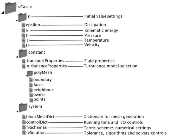
Therefore, any OpenFOAM case must contain the following directories and these are further discussed in detail in the upcoming sub-sections

• constant

• 0 (Zero)

• system

constant directory

The files in the constant directory usually include files that provide information about constants that are used in the project. This include material properties, turbulence properties etc. In the directory polyMesh, the mesh data are stored (in this case the data for converted mesh). The boundary file in this polyMesh directory includes the mesh boundary data, e.g. type, the patch group, number of faces on this boundary and also starting face number (unique face IDs) for this boundary, e.g. transportProperties.

0 (Zero) directory

The 0 directory includes the initial conditions for running the simulation. In each file in this folder the initial conditions for one property can be set.

Time directories

The time directories appear in the case file after the case is simulated. It can also be used specify initial conditions. The solution files contain solved data for particular fields, e.g. velocity, temperature, pressure. The data contained are results written to file by OpenFOAM. For example, in the cavity tutorial, the velocity field and pressure fields are initialized from files 0/U and 0/p respectively.

system directory

This directory is for setting parameters associated with the solution procedure itself. It contains at least the following three files:

• fvSchemes: The discretization scheme which is used for each term of the equations are set in this file.

• fvSolution: This contains the settings to the coupling method of pressure and velocity, the numerical methods, which are used for solving different quantities, and also the final tolerance for convergence of that quantity.

• controlDict: The controlDict dictionary is used to specify the main case controls. This includes, e.g. timing information, write format, and optional libraries that can be loaded at run time.

OpenFOAM files

Let us continue to look at the functionality of each file in the OpenFOAM directory. Of particular interest are the files in the system and control directories since these files control the flow of the simulation. We will particularly address the mesh files in the upcoming lectures.

system/fvSolution file

The fvSolution file includes the description of solvers, smoothers and relaxation factors. Here solvers refer to the methods that are used to solve the final matrix equations that are obtained from the discretization of the original differential equations. In this regard, there are direct and iterative solvers that can be utilized. Most often, these solvers need pre-processing before the system of equations can be solved. Here, pre-conditioners improve the condition numbers, smoothers reduce the number of iterations required to solve, tolerances are specified to provide value at which convergence is achieved. Thus, the methods required for the pre-conditioners, smoothers and tolerances also need to be provided along with the information about a solver.

The syntax for each entry within solvers starts with a keyword that is of the variable being solved in the particular equation. For example, icoFoam solves equations for velocity and pressure, hence contains the entries for velocity U and pressure p. The keyword relates to a sub-dictionary containing the type of solver and the parameters that the solver uses. If the user specifies a symmetric solver for an asymmetric matrix, or vice versa, an error message will be written to advise the user accordingly. The following solvers are used for the present version in OpenFOAM:

• PCG/PBiCGStab: Stabilised preconditioned (bi-)conjugate gradient solver, for both symmetric and asymmetric matrices.

• PCG/PBiCG: Preconditioned (bi-)conjugate gradient, with PCG for symmetric matrices, PBiCG for asymmetric matrices.

• smoothSolver: solver that uses a smoother. This also requires a smoother to be provided. Some of the smoothers include GaussSeidel, symGaussSeidel, DIC/DILU

• GAMG: The generalized method of Geometric-Algebraic Multi-Grid (GAMG) solvers are faster than standard methods. They solve a solution on a coarser mesh, map this solution onto a finer mesh and then use the mapped solution as a first approximation. Here, GAMG starts with the mesh specified by the user and automatically coarsens or refines the mesh. There are several options available for the GAMG solvers that control the agglomeration of cells. The primary ones include:

  • cacheAgglomeration: A switch to specify caching of the agglomeration strategy (default true)

  • nCellsInCoarsestLevel: Approximate mesh size at the coarsest level (default 10)

  • directSolveCoarset: Switch to use a direct solver at the coarsest level (default false)

  • mergeLevels: It controls the speed and number of levels to be refined at a time (default 1)

As discussed earlier, when iterative solvers are used, a pre-conditioner is needed to improve the solvability of the system of matrix equations. Pre-conditioning is the application of a transformation, called the pre-conditioner, that conditions a given problem into a form that is more suitable for numerical solving methods. Pre-conditioning is typically related to reducing a condition number of the problem. The pre-conditioned problem is then usually solved by an iterative method. A preconditioned iterative solver solves the system \([M]^{-1}[A]{x} = [M]^{-1}{b}\) with \(M\) being the pre-conditioner. The chosen pre-conditioner should ensure that convergence for the preconditioned system is much faster than for the original one. In simple terms, the pre-conditioner leads to a faster propagation of information through the mesh. The pre-conditioners available in OpenFOAM include:

• DICPreconditioner: A simplifed diagonal-based incomplete Cholesky preconditioner for symmetric matrices (symmetric equivalent of DILU). The reciprocal of the preconditioned diagonal is calculated and stored

• DIC/DILU: Diagonal incomplete-Cholesky (symmetric) and incomplete-LU (asymmetric)

• GAMG: geometric-algebraic multi-grid

• none: no preconditioning

Although the preconditioners can considerably reduce the number of iterations, they do not normally reduce the mesh dependency of the numbers of iterations. OpenFOAM supplies the following smoothers to be used with the solvers and the choice of smoother to be specified. The smoother options are listed below. The symGaussSeidel and GaussSeidel smoothers are often suitable for general problems and used extensively in the OpenFOAM tutorials. Tohers include, DIC/DILU and DICGaussSeidel. On aspect to note is that when using the smooth solvers, the user can optionally specify the number of sweeps, by the nSweeps keyword, before the residual is recalculated.

Since the solvers are generally iterative, in nature, we need to further specify when the convergence has been reached. Numerically, we will never reach a zero but reach thresholds like \(10^{-4}, 10^{-8}, 10^{-16}\) and so on. Thus, we need to specify a small number when we can say the convergence has been reached. This is done by specifying the tolerance for the residual. The residual is the measure of the error in the solution. Ideally, it is expected that after each solver iteration, the residual is re-evaluated and is smaller than that of the previous iteration. A solver eventually stops when one of the below three conditions are met:

• The residual falls below the solver tolerance

• The ratio of the current to the initial residuals falls below the solver’s relative tolerance relTol

• The number of iterations exceeds a maximum number of iterations maxIter

The solver tolerance should represent the level at which the residual is small enough that the solution can be deemed sufficiently accurate. The solver relative tolerance limits the relative improvement from initial to final solution. Most fluid dynamics solver applications in OpenFOAM use either the pressure-implicit split-operator PISO, the semi-implicit method for pressure-linked equations SIMPLE algorithms, or a combined PIMPLE algorithm. Equations are very often solved multiple times within one solution step, or time step. For example, when using the PISO algorithm, a pressure equation is solved according to the number specified by nCorrectors.

The relaxationFactors controls the stability of a computation, particularly in solving steady-state problems. Relaxation factors play a vital role in determining the rate of convergence for CFD simulation. When the relaxation factor is less than one it is said to be under relaxed else it is called over relaxed. When the under relaxed values are applied to the successive iterations of the point iterative techniques such as Gauss-Seidel method, the convergence rate of the solution increases. We will discuss the topic of relaxation further in the advanced tutorials.

The last topic is of pressure referencing. In a closed incompressible system, the pressure is relative. In otherwords, it is the pressure range that matters not the absolute values. In these cases, the solver sets a reference level equal to pRefValue in the cell pRefCell. These entries are generally stored in the SIMPLE, PISO or PIMPLE sub-dictionaries and are used by those solvers that require them when the case demands it. We will again address these issues later in the advanced tutorials.

system/fvSchemes file

The fvSchemes file in the system directory sets the numerical schemes for terms, such as derivatives in equations, that are calculated during a simulation. Before going into the layout of fvSchemes, it is essential to understand how OpenFOAM accepts or takes inputs of partial differential equations. A central theme of the OpenFOAM design is that the solver applications, written using the OpenFOAM classes, have a syntax that closely resembles the partial differential equations being solved. For example, the equation

\[\frac{\partial \rho U }{\partial t} + \nabla \cdot \phi - \nabla \cdot \mu \nabla U = - \nabla p\]

is represented by the code,

solve
(
    fvm::ddt(rho, U)
  + fvm::div(phi, U)
  - fvm::laplacian(mu, U)
    ==
  - fvc::grad(p)
);

The set of terms, for which numerical schemes must be specified, are subdivided within the fvSchemes file into the categories below. Each keyword in represents the name of a sub-dictionary which contains terms of a particular type.

• timeScheme: First and second time derivatives, e.g. ddt for \(\frac{\partial }{\partial t}\)

• gradSchemes: Gradient terms, e.g., grad(p), which represents \(\nabla p\)

• divSchemes: Divergence terms

• laplacianSchemes: Laplacian terms

• interpolationSchemes: Cell to face interpolations of values

• snGradSchemes: Component of gradient normal to a cell face

• wallDist: Distance to wall calculation.

A sample file of the fvSchemes is shown below to illustrate various schemes

If a default scheme is specified in a particular Schemes sub-dictionary, it is assigned to all of the terms in the sub-dictionary except those terms that are explicitly specified otherwise. We can also specify that no default scheme by the none entry. In this section, only the time schemes are discussed. The first time derivative \(\left( \frac{\partial }{\partial t} \right)\) terms are specified in the ddtSchemes sub-dictionary. The discretization schemes for each term can be selected from those listed below.

• steadyState: sets time derivatives to zero.

• Euler: transient, first order implicit, bounded.

• backward: transient, second order implicit, potentially unbounded.

• CrankNicolson: transient, second order implicit, bounded; requires an off-centering coefficient

• localEuler: pseudo transient for accelerating a solution to steady-state using local-time stepping; first order implicit.

It is important to note here that for any second-order time derivative \(\frac{\partial ^ 2 }{\partial t^2}\) terms, only the Euler scheme is available for d2dt2Schemes.

system/controlDict file

The last important file is the controlDict. This controls all the simulation parameters like start and stop times, time interval, time interval for writing outputs and so on.

The controlDict dictionary sets input parameters essential for the creation of the database.

• startFrom : This function controls the start time of the simulation.

• startTime: It is the numerical value of the start time for the simulation.

• stopAt: This function controls the end time of the simulation.

• endTime: It is the End time for the simulation when stopAt endTime.

• deltaT: It is the Time step of the simulation.

• writeControl: This function controls the timing of write output to file.

• writeInterval: This function is a scalar which is used in conjunction with writeControl.

• timeStep: It writes data every writeInterval time steps.

• purgeWrite: It is an integer representing a limit on the number of time directories that are stored by overwriting time directories on a cyclic basis.

• writeFormat: It specifies the format of the data files.

• Ascii: ASCII format, written to writePrecision significant figures.

• writePrecision : It is an integer used in conjunction with writeFormat, 6 by default.

• writeCompression: Switch to specify whether files are compressed with gzip when written: on/off.

• timeFormat: It is the choice of format of the naming of the time directories.

• general: Specifies scientific format if the exponent is less than -4 or greater than or equal to that specified by timePrecision.

• timePrecision: It is an integer used in conjunction with timeFormat , 6 by default.

• runTimeModifiable: Switch for whether dictionaries, e.g. controlDict, are re-read during a simulation at the beginning of each time step, allowing the user to modify parameters during a simulation.

Other case files

The other case files present in the tutorial directory for a case are transportProperties, turbulenceProperties stored in the constant sub directory and initial conditions such as initial pressure and velocity magnitude stored in the 0 sub directory. More information about these files will be discussed in the coming lectures.

OpenFOAM Solvers

While the word solvers is used often and interchangeably in the context of OpenFOAM literature, it should be noted here that we are talking here about a workflow that has been designed to solve a specific genre of problem in computational continuum mechanics. OpenFOAM does not have a generic solver applicable to all types of problems. Instead, users must choose a specific solver for a class of problems to solve. There are flow Solvers as well as non-flow (other) solvers present in the package. The flow solvers include:

• Basic

• Incompressible

• Compressible

• Heat transfer

• Multiphase

• Lagrangian particles

• Discrete methods

• Combustion

• DNS

and the non-flow solver includes, those applicable for

• Electromagnetics

• Financial

• Stress analysis

There are a slew of solvers available. The summary of capabilities of the solvers are as given in the table below. In the next subsections, we will look at a comprehensive list of solvers available and their utility value.

Solver	Transient	Compressible	Turbulence	Dynamic Mesh
boundaryFoam
icoFoam	X
pimpleFoam	X		X	X
laplacianFoam	X
pisoFoam	X		X
simpleFoam			X
sonicFoam	X	X	X

Basic solvers

• laplacianFoam: Solves a simple Laplace equation, e.g. for thermal diffusion in a solid

• potentialFoam: Potential flow solver which solves for the velocity potential, to calculate the flux-field, from which the velocity field is obtained by reconstructing the flux

• scalarTransportFoam: Solves the steady or transient transport equation for a passive scalar

Incompressible flow solvers

• boundaryFoam: Steady-state solver for incompressible, 1D turbulent flow, typically to generate boundary layer conditions at an inlet, for use in a simulation.

• icoFoam: Transient solver for incompressible, laminar flow of Newtonian fluids.

• pimpleFoam: Transient solver for incompressible, turbulent flow of Newtonian fluids, with optional mesh motion and mesh topology changes.

• pisoFoam: Transient solver for incompressible, turbulent flow, using the PISO algorithm.

• simpleFoam: Steady-state solver for incompressible, turbulent flow, using the SIMPLE algorithm.

Compressible solvers

• sonicFoam: Transient solver for trans-sonic/supersonic, turbulent flow of a compressible gas.

• rhoPimpleFoam: Transient solver for turbulent flow of compressible fluids for HVAC and similar applications, with optional mesh motion and mesh topology changes.

• rhoSimpleFoam: Steady-state solver for turbulent flow of compressible fluids.

Utilities and Libraries

Utilities are tools that aid in pre-processing, mesh generation, mesh manipulation, post processing and other miscellaneous activities. They perform simple pre-and post-processing tasks mainly involving data manipulation and algebraic calculations and meshing. For example, checkMesh checks the validity of a mesh. Each application is designed to be executed from a terminal command line, typically reading and writing a set of data files associated with a particular case. The data files for a case are stored in a directory named after the case.

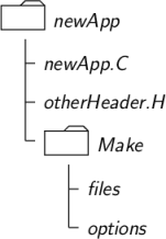
Together, the solver and the associated utilities are involved in the working of an application. OpenFOAM applications are organized using a standard convention that the source code of each application is placed in a directory whose name is that of the application. The top level source file then takes the application name with the .C extension. For example, the source code for an application called newApp would reside is a directory newApp and the top level file would be newApp.C as shown in the figure below.

Additionally, OpenFOAM is divided into a set of pre-compiled libraries that are dynamically linked during compilation of the solvers and utilities. OpenFOAM includes an extensive collection of library functionality covering most aspects engineering flow problems such as physical modeling, boundary conditions, numerics and mesh motion. Libraries such as those for physical models are supplied as source code so that users may conveniently add their own models to the libraries.