Lecture 03: Boundary conditions
The accurate treatment of boundary conditions is critical in many computational fluid dynamics (CFD) simulations. Fundamentally, problems associated with boundary conditions for compressible flows arise because of the difficulty in ensuring a well-posed problem. Each boundary condition has a physical meaning described mathematically via an equation, which in the context of a numerical method has to be translated into an algebraic relation. An inlet boundary condition for instance, describes a known flow behavior where velocity and pressure satisfy specified physical conditions. These include a Dirichlet and a Neumann condition, which should be defined in order to connect the mathematical model with the boundary conditions of the problem. This lecture gives an insight into the boundary conditions in and their implementation in OpenFOAM.
In order to accomplish this task, we need to briefly discuss the Navier stokes equations. In this regard, let us consider the equations for the conservation of mass, momentum and energy.
Conservation relations
Mass conservation
The law of mass conservation or the law of continuity establishes the fact that mass cannot be created in such a closed fluid system, nor can disappear from it. There is also no diffusive flux contribution to the continuity equation, since for a fluid at rest, any variation of mass would imply a displacement of fluid particles. The conserved quantity in this case is the density \(\rho\). For the time rate of change of the total mass inside the control volume \(\Omega\) we have,
The mass flow of a fluid through some surface fixed in space equals to the product of density, surface area and velocity component perpendicular to the surface. Therefore, the contribution from the convective flux across each surface element \(dS\) becomes,
Since there are no source terms present, we can write this as
This represents the integral form of the continuity equation - the conservation law of mass.
Momentum Conservation
The variation of momentum is caused by the net force acting on an mass element. For the momentum of an infinitesimally small portion of the control volume \(\Omega\),
The variation in time of momentum within the control volume equals,
Hence, the conserved quantity is here the product of density times the velocity, i.e.,
The convective flux tensor, which describes the transfer of momentum across the boundary of the control volume, consists in the Cartesian coordinate system of the following three components.
x- component : :math`rho u vec{v}`
y- component : :math`rho v vec{v}`
z- component : :math`rho w vec{v}`
The contribution of the convective flux tensor to the conservation of momentum is then given by
The diffusive flux is zero, since there is no diffusion of momentum possible for a fluid at rest. There also exists a body force per unit volume, denoted as \(\rho f_e\) corresponds to the volume sources in. Thus, the contribution of the body (external) force to the momentum conservation is
The surface sources consist then of two parts - an isotropic pressure component and a viscous stress tensor \(\tau\),
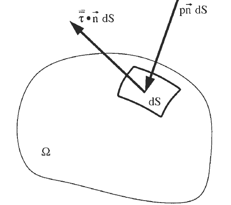
Forces acting on the surface of an element in the control volume
Summing up all the above contributions, we finally obtain the expression,
for the momentum conservation inside an arbitrary control volume \(\Omega\) which is fixed in space.
Energy Conservation
Any changes in time of the total energy inside the volume are caused by the rate of work of forces acting on the volume and by the net heat flux into it. The total energy per unit mass E of a fluid is obtained by adding its internal energy per unit mass, \(e\), to its kinetic energy per unit mass, \(\frac{v^2}{2}\). Thus, we can write for the total energy,
The conserved quantity is in this case the total energy per unit volume, i.e., \(\rho E\). Its variation in time within the volume :math`rho` can be expressed as,
The contribution of the convective flux can then be written as,
In contrast to the continuity and the momentum equation, there is now a diffusive flux. The diffusion flux represents the diffusion of heat due to molecular thermal conduction - heat transfer due to temperature gradients. Therefore, writing it in the form of Fourier’s law of heat conduction,
with \(k\) standing for the thermal conductivity coefficient and \(T\) for the absolute static temperature. The final addition to the momentum equation will be the source terms: both volume and surface source terms. Surface source terms correspond to the time rate of work done by the pressure as well as the shear and normal stresses on the fluid element. The volume source terms contains the time rate of heat transfer per unit mass - as \(q_h\) and the rate of work done by the body forces \(f_e\). These can be written as the following,
Gathering all the terms involved we finally obtain,
where,
Boundary treatment methods
To get a consistent unique solution for a specific problem, it is imperative to define the boundary conditions. However, before delving into that section we must understand how boundaries are treated in order to completely grasp the concept of boundary conditions. Boundary treatments are usually an issue when/if the chosen spatial approximation requires the value of the solution at non-existing points . Typical boundary treatments either
Change the approximation method at the edge, i.e; one-sided approximations
Change the computational domain at the edge, i.e; ghost cells.
Normally, a numerical scheme involves a certain “stencil” of cells from one or both sides of the cell solved for. But, in finite volume method, when we reach the edge of the computational domain, the scheme for the interior cannot be applied since there are no neighboring cells to solve for the stencil. For example, we cannot use central differencing cannot be applied to cells at the boundary because they do not have any cells preceding them. Thus, for boundary cells, the original numerical scheme applied for the interior cells needs to be changed. The disadvantage of such method is that the solution algorithm needs to be altered around the boundaries, which increases the coding complexity.
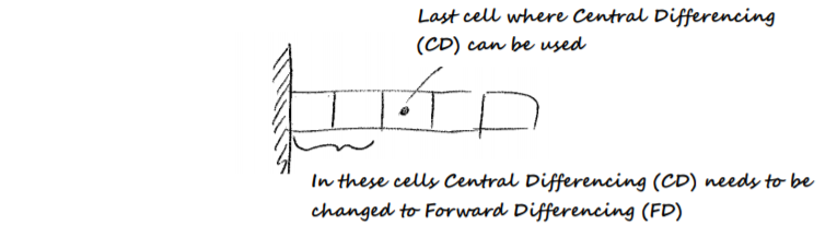
Constraint at boundaries - change of numerical approximation method at boundaries is required
Another alternative is to change the computational domain by introducing so called “ghost cells” outside of the boundary. Usually, 1 or 2 layers of ghost cells are introduced, depending on the size of the stencil. The advantage of the ghost cell method is that the numerical scheme used for the interior can be used unaltered for the boundaries. The idea is to introduce fictitious flow in the ghost cells which will yield the desired boundary conditions on the edge.
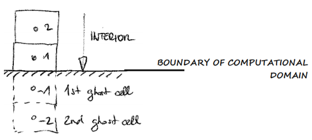
Ghost Cell Approach at Boundaries, which eliminates the need to change numerical approximation method at boundaries alone
Types of boundaries
An appropriate specification of boundary conditions is very important to solve any problem in CFD as it helps model the numerical solution in closeness to real world problems. Boundaries direct motion of flow and specify fluxes their direction in the computational domain, e.g.mass, momentum, energy or any other physical property. Defining boundary conditions involves two main steps:
Identifying the location of the boundaries (e.g., inlets, walls, symmetry)
Supplying information at the boundaries
In OpenFOAM or any other commercial flow solver, boundaries and internal surfaces are represented by face zones. Boundary data, material and source terms are then assigned to these face zones. It is essential to note that for different variables, different kinds of boundary conditions may be defined for the same boundary.The major classification of boundary conditions in the field of CFD are described below.
Neumann and Dirichlet
This is the most fundamental classification of boundary conditions. Neumann and Dirichlet boundary conditions can be distinguished better mathematically rather than descriptively. Dirichlet boundary condition directly specifies the value of a variable at the boundary, e.g. u(x) = constant. While for Neumann boundary condition, the gradient normal to the boundary of a variable at the boundary needs to be specified. There also exists another boundary condition called the mixed boundary condition which is a combination of both Neumann and Dirichlet conditions. This is of the form,
Free and Solid surfaces
This is the flow, which would occur if the computational domain would be completely “empty,” i.e. free of any solid objects. If a solid object is present in the computational domain, then freestream conditions would occur at infinite distance from the solid object. Free surfaces are either far-field boundaries in external flows or inlet and outlet sections of internal flow systems. These are the boundaries through which the flow enters or leaves the computational domain. In external flow problems, free boundaries are generally located far enough from the body such that free-stream conditions can be considered. Farfield boundary is a case such that the boundary is at finite distance from the solid object, with values slightly different than the freestream values would be. The numerical simulation of external flows past airfoils, wings, cars and other configurations has to be conducted within a bounded domain. For this reason, artificial farfield boundary conditions have been introduced. The implementation of the farfield boundary conditions for a flow problem has two prerequisites: First, the truncation of the domain should have no notable effects on the flow solution as compared to the infinite domain. Second, any outgoing disturbances must not be reflected back into the flow field. Usually, we do not know the far-field values, but only the freestream ones. But, we need to set some values for the far-field, so we set the freestream values for these. Let us consider the flow conditions shown below. On the left, we have an inflow and on the right, an outflow.
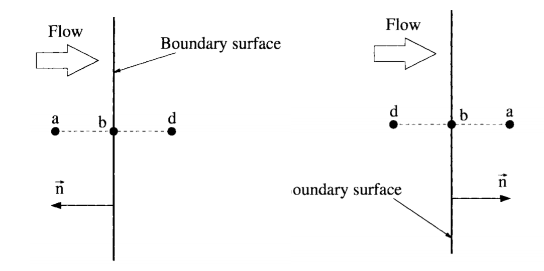
Farfield boundary:inflow (left); Farfield boundary:outflow (right)
In the above scenario, the position a is outside, b on the boundary, and position d is inside the physical domain. The unit normal vector \(n = [n_z, n_y, n_z]^T\) points out of the domain. Depending on the local Mach number, four different types of farfield boundary conditions have to be treated:
Supersonic inflow
Supersonic outflow
Subsonic inflow
Subsonic outflow
Alternatively, in internal flow systems, these are simply referred to as the inlet and outlet surfaces as * Subsonic inlet * Subsonic outlet
In the case of walls, they can be represented as * Solid walls: Inviscid and viscous flow * Moving wall
Boundary conditions that account for the symmetries and periodicities are: * Periodic * Symmetric plane
Supersonic inflow
For supersonic inflow, the conservative variables on the boundary are determined by freestream values only as
This basically translates to,
The values \(\vec{W_a}\) are specified based on the given Mach number \(M_\infty\) and on two flow angles.
Subsonic inflow
In subsonic inflow, four characteristic variables are prescribed based on the freestream values. One characteristic variable is extrapolated from the interior of the physical domain. This leads to the following set of boundary conditions:
where \(p_0\) and \(c_0\) represent a reference state. The reference state is normally set equal to the state at the interior point(8d*). The values in point a are determined from the freestream state.
Subsonic Outflow
In the case of subsonic outflow, four flow variables (density and the three velocity components) have to be extrapolated from the interior of the physical domain. The remaining fifth variable (pressure) must be specified externally. The primitive variables at the farfield boundary are obtained from
with \(p_a\) being the prescribed static pressure. Physical properties in the ghost cells can be obtained by linear extrapolation from the states :math`b` and \(d\).
Subsonic Inlet
A common procedure consists of the specification of the total pressure, total temperature, and of two flow angles. One characteristic variable has to be interpolated from the interior of the flow domain. One possibility is to employ the outgoing Riemann invariant which is defined for an ideal gas as,
where the index d denotes the state inside the domain. The Riemann invariant is used to determine either the absolute velocity or the the speed of sound at the boundary. In practice, it was found that selecting the speed of sound leads to a more stable scheme, particularly for low Mach-number flows. Therefore, we express the speed at boundary using flow angles, \(\gamma\) (specific heat ratio) and the total velocity at the interior point \(d\). Quantities like the static temperature, pressure, density, or the absolute velocity at the boundary are evaluated as follows
where \(T_0\) and \(p_0\) are the given values of total temperature and pressure, \(R\) and \(C_p\) represent the specific gas constant and the heat coefficient at constant pressure, respectively. The velocity components at the inlet are obtained by decomposing \(||\vec{v_b||\) according to the two (one in 2D) prescribed flow angles.
Subsonic Outlet
The subsonic outflow condition specifies the static pressure, and extrapolates density and velocity. The subsonic outlet boundary can be treated in a way quite similar to the outflow condition for farfield flows. Only the ambient pressure \(p_a\) is replaced here by the given static exit pressure.
Solid Wall: Inviscid flow
In the case of an inviscid flow, the fluid slips over the surface.
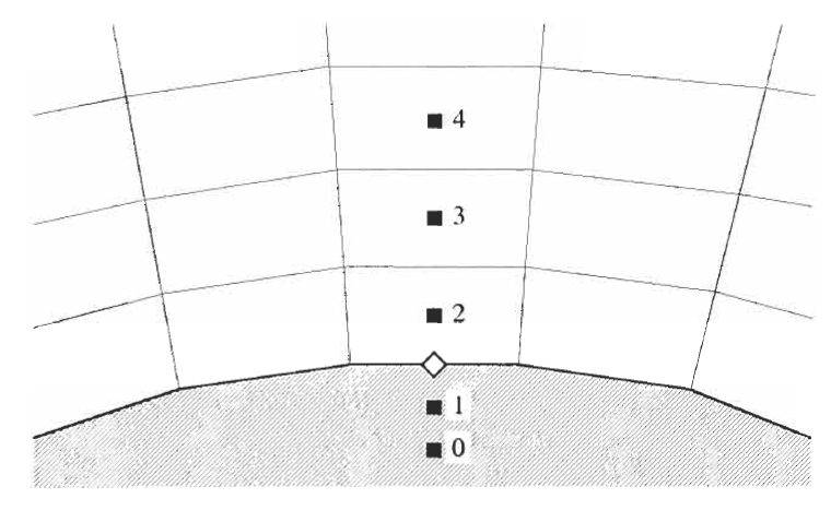
Solid wall boundary depicting ghost cells, here 0 and 1
Since there is no friction force, the velocity vector must be tangent to the surface. This is equivalent to the condition that there is no flow normal to the surface, Hence,
where \(\vec{n}\) denotes the unit normal vector at the surface. Hence, the contravariant velocity \(V\) is zero at the wall. Consequently, the vector of convective fluxes reduces to the pressure term alone, i.e,
with \(p_w\) being the wall pressure. Within the cell-centred scheme, the pressure is evaluated at the centroid of the cell. We can obtain the wall pressure most easily by extrapolation from the interior of the domain. As shown in the above figure, we could simply set \(p_w\) = \(p_2\). Higher accuracy is achieved using either a two-point extrapolation,
or a three point extrapolation,
Viscous Flow
For a viscous fluid which passes a solid wall, the relative velocity between the surface and the fluid directly at the surface is assumed to be zero. Therefore, we speak of noslip boundary condition. In the case of a stationary wall surface, the Cartesian velocity components become,
The implementation of the noslip boundary condition, it can be simplified by the utilization of ghost cells. In the case of an adiabatic wall (i.e. no heat flux through the wall), we can set
and likewise for the cells 0 and 3 in the domain.
Moving Wall
For any point of the fluid boundary layer adjacent to a solid wall moving with a certain velocity, we can write the following relations,
where \(wall,A\) stands for wall velocity at the point A on solid wall surface.
Periodic Boundaries
This boundary is established when physical geometry of interest and expected flow pattern and the thermal solution are of a periodically repeating nature. This reduces computational effort in our problems. Consider the figure shown below
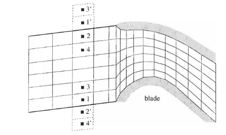
Periodic Boundary sketch depicting the repetitive cells
The configuration is periodic in the vertical direction. The shaded cells 1 and 2 are located on the lower and the upper periodic boundary, respectively. Due to the periodicity condition, the first ghost-cell layer corresponds to the boundary cells at the opposite periodic boundary. The second ghost-cell layer communicates with the second layer of the physical cells and so on. Hence, all scalar quantities (density, pressure, etc.) in the ghost cells are obtained directly from the corresponding physical cells. Hence, we can write,
The same relations hold also for the vector quantities (velocity, gradients) in this case.
Symmetric Plane
If the flow is to be symmetrical with respect to a line or a plane, the following conditions must be met:
No flux across the boundary
Gradient of a scalar quantity normal to the boundary,
Gradient of the tangential velocity normal to the boundary,
Gradient of the normal velocity along the boundary (since \(\vec{v} \cdot \vec{n} = 0\))
These can be translated to mathematical expressions as,
The implementation of the symmetry boundary condition can be largely simplified by employing ghost cells. The flow variables in the ghost cells are obtained using the concept of reflected cells. This means that scalar quantities like density or pressure in the ghost cells are set equal to the values in the opposite interior cells, i.e., \(U_1 = U_2\) and \(U_0 = U_3\). The velocity components are reflected with respect to the boundary.
Boundary conditions in OF
In OpenFOAM, for the purpose of applying boundary conditions, a boundary is generally broken up into a set of patches. One patch may include one or more enclosed areas of the boundary surface which do not necessarily need to be physically connected. A type is assigned to every patch as part of the mesh description. Every patch includes a type entry that specifies the type of boundary condition and a value to specify the value of the variable at the boundary condition. They range from a basic fixedValue condition applied to the inlet, to a complex waveTransmissive condition applied to the outlet. The patches with non-generic types, e.g. symmetryPlane, defined in boundary, use consistent boundary condition types in the p file.
The main geometric types available in OpenFOAM are summarized below.
patch: generic type containing no geometric or topological information about the mesh, e.g. used for an inlet or an outlet.wall: for patch that coincides with a solid wall, required for some physical modeling, e.g. wall functions in turbulence modeling.symmetryPlane: for a planar patch which is a symmetry plane.symmetry: for any (non-planar) patch which uses the symmetry plane (slip) condition.empty: for solutions in in 2 (or 1) dimensions (2D/1D), the type used on each patch whose plane is normal to the 3rd (and 2nd) dimension for which no solution is required.wedge: for 2 dimensional axis-symmetric cases, e.g. a cylinder, the geometry is specified as a wedge of small angle and 1 cell thick, running along the centre line, straddling one of the coordinate planes, the axis-symmetric wedge planes must be specified as separate patches ofwedgetype.
Boundary conditions in OpenFOAM are divided into two groups by - basic and derived. The main basic boundary condition types available in OpenFOAM are summarised below using a patch field named \(Q\)
fixedValue: value of \(Q\) is specified by value(Dirichlet).fixedGradient: normal gradient of \(Q\), that is \(\frac{\partial Q}{\partial n}\) is specified by gradient(Neumann).zeroGradient: normal gradient of \(Q\) is zero.calculated: patch field \(Q\) calculated from other patch fields.mixed: mixedfixedValue/fixedGradientcondition depending onvalueFraction\((0 \leq valueFraction \leq 1)\)directionMixed: mixed condition with tensorial valueFraction, to allow different conditions in normal and tangential directions of a vector patch field, e.g. fixedValue in the tangential direction, zeroGradient in the normal direction.
There are numerous more complex boundary conditions derived from the basic conditions. For example, many complex conditions are derived from fixedValue, where the value is calculated by a function of other patch fields, time, geometric information, etc. Some other conditions derived from mixed / directionMixed switch between fixedValue and fixedGradient. These are not discussed currently here but will be later addressed in the advanced modules.
In OpenFOAM, almost all definitions of boundary conditions are stored in the following directory: src/finiteVolume/fields/fvPatchFields``with the main implemented ``types of boundary conditions stored in the subdirectories listed below:
basic
constraint
derived
fvPatchField
The fvPatchField directory contains the general class definition of a boundary condition, which represents the base class. This class defines the main functions and data structures that will be used and will be inherited by the genuine classes. The basic directory contains the basic mathematically defined boundary conditions including the Dirichlet type ( fixedValue`), the Neuman type ( zeroGradient/fixedGradient) and the Robin type ( mixed) boundary conditions. An additional entry included in basic directory is the coupled boundary condition that implements a patch to patch type condition, i.e., coupling two boundary patches together (coupled boundaries). The constraint directory contains geometric type boundary conditions that derive from the coupled boundary class. An example is the periodicity boundary condition. Finally the derived directory includes all boundary conditions that are derived from the basic boundary conditions. These derived boundary conditions are simply specializations of the basic types.