2.3. SIM: Structural Model
The user here defines the structural system of the building. The structural system is the part of the building provided to resist the gravity loads and those loads arising from the natural hazard. There are a number of backend applications provided for this part of the workflow, each responsible for defining the structural analysis model. The user can select the application to use from the drop-down menu at the top of this panel. As the user switches between applications, the input panel changes to reflect the inputs each particular application requires. At present, there are a few backend applications available.
2.3.1. Multiple Degrees of Freedom (MDOF)
This panel is provided for users to quickly create simple shear models of a building. The panel, as shown in Fig. 2.3.1.1 is divided into 3 frames:
The top left frame allows the user to specify the number of stories and properties that are constant for every floor and story in the building. The following properties are available: floor weight, story height, torsional stiffness, initial stiffness, yield strength, and hardening ratio for each direction in each story. The user has the option of specifying values for eccentricity of mass in \(x\) and \(y\) directions, and eccentricities for the location of the response quantities. Here, the one and two directions are orthogonal \(x\) and \(y\) axes in plan view.
The lower left frame allows the user to override the structural parameters above for individual floors and stories.
The frame on the right is a graphical widget showing the current building. When entering data into the lower left frame, the stories corresponding to the data being modified are highlighted in red.
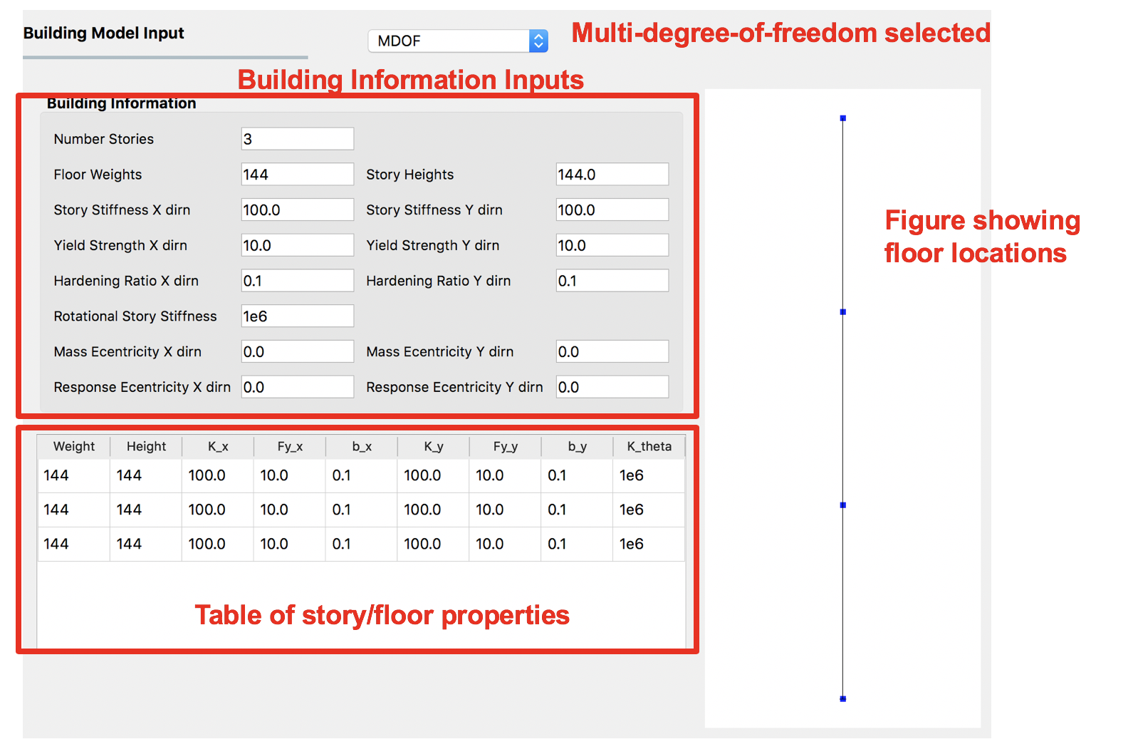
Fig. 2.3.1.1 Multiple degrees of freedom (MDOF) building model generator.
Random variables can be created by the user if they enter a valid string instead of a number in the entry fields for any entry except for the Number of floors. The variable name entered will appear as a random variable in the RV panel; it is there that the user must specify the distribution associated with the random variable.
2.3.2. OpenSees
This panel is for users who have an existing OpenSees model of a building that performs a gravity analysis and now they wish to subject that building model to one of the EVT options provided. The input panel for this option is shown in Fig. 2.3.2.1. Users need to provide three pieces of information:
Main OpenSees Script: The main script that contains the building model. This script should build a model and perform any gravity analysis of the building that is required before the event is applied.
Response Nodes: A list of node numbers that define a column line of interest for which the responses will be determined. The column nodes should be in order from ground floor to roof. The EDP workflow application uses this information to determine nodes at which displacement, acceleration, and story drifts are calculated.
An entry for the dimension of the model (i.e., 2D or 3D). This information is used when loads are applied.
Entry for the number of degrees of freedom at each node in the model.

Fig. 2.3.2.1 OpenSees Model.
In OpenSees there is an option to set a variable to have a certain value using either the set or pset command, e.g pset a 5.0 will set the variable a to have a value 5 in the OpenSees script. In EE-UQ, any variable found in the main script to be set using the pset command will be assumed to be a random variable. As such, when a new main script is loaded, all variables set with pset will appear as random variables in the UQ panel.
2.3.3. Steel Building Model (AutoSDA)
This module provides a way for a user to create a nonlinear structural model of a moment-resisting steel-framed building. The AutoSDA computer program [GBS20] is used for the seismic design and to generate the resulting two-dimensional structural model in OpenSees. AutoSDA automates the seismic design process and nonlinear structural model construction, generating code-conforming section sizes and detailing for beams, columns, and beam-column connections based on the user-specified input design parameters. The resulting nonlinear model is then subjected to the hazard option that is selected by the user in the EVT panel. The TCL files of the OpenSees model generated by AutoSDA are located in the individual work directories in the tmp.SimCenter folder that EE-UQ creates on the user’s computer.
The input panel for this module is shown in Fig. 2.3.3.1. Users need to provide the following information:
Building Information Inputs: The building information box describes the building geometry. The units for the building geometry parameters are in feet. Changing the building parameter values will update the building properties in the GI panel. Also, changing the number of building stories will add or subtract rows from the
Member DepthandLoadingtables below.Seismic Design Parameters: The seismic design parameters box contains the Equivalent Lateral Force (ELF) design parameters as specified by ASCE 7-10. AutoSDA employs these parameters in its automated seismic design procedures. Note that the values of these ELF parameters are site-specific, and can be obtained from the SEAOC/OSHPD Seismic Design Maps Tool or the ATC Hazards by Location Tool.
Building Data Folder: The location of the building data folder is specified within this box. The building data folder should contain the following four CSV files that are required by AutoSDA: 1) Geometry.csv; 2) ELFParameters.csv; 3) MemberDepth.csv; and 4) Loads.csv. These files can be automatically created on the user’s computer by clicking on the
Save Filebutton. The user will be prompted to select a folder whereafter the files will be saved. Alternatively, users have the option to upload their own CSV files by selecting a folder, and then clicking on theLoad Filebutton. Note that users are encouraged to backup their CSV files as EE-UQ will overwrite the existing files in the selected folder. Before running an analysis, users must save or load the corresponding CSV files so that AutoSDA can locate them.Member Depth Table: This table lists the user-specified depths for the interior columns, exterior columns, and beams. Each row in the table corresponds to a building story. The first row corresponds to the first story, the second row to the second story, etc. As shown in Fig. 2.3.3.1, the member depth values need to follow nomenclature from the AISC steel shapes database, e.g., W14, W24. If multiple depths are specified, the depths need to be separated by a comma, followed by a space.
Loading Table: This table contains the loading values for the floors, beams and columns. As in the
Member Depthtable, each row in this table corresponds to its own building story. In this table, there is an option to specify the loading values as random variables. This is done by entering a unique name tag for a random variable in lieu of a numerical value. For example, in any of the cells in the table, a user can enter the textSomeRV.TheSomeRVrandom variable tag will then appear in the UQ panel, where the type of distribution, mean value, etc., can be specified.
Warning
When employing the AutoSDA building model, the analysis may not converge with the default settings in the FEM tab. The user should change the convergence test in the FEM tab to be: EnergyIncr 1.0e-3 300
Note
If the CSV files in the building data folder are modified by hand, the top-most headings in the CSV files should not be changed. AutoSDA will not recognize the headings if they are altered, and thus the required data will not get imported. Moreover, the number of rows in the MemberDepth.csv and Loads.csv files needs to match the number of building stories in the Geometry.csv file.
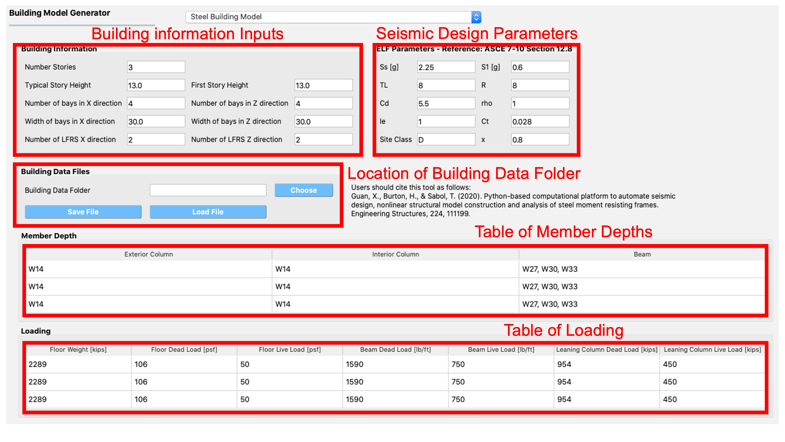
Fig. 2.3.3.1 Steel Building Model.
2.3.4. Concrete Building Model (RC-FIAP)
This module provides a way for a user to create a nonlinear structural model of a reinforced concrete building. The RC-FIAP (Reinforced Concrete Frame Inelastic Analysis Platform) computer program generates a two-dimensional structural model that is employed in OpenSees. RC-FIAP automates the seismic design process and inelastic structural model construction based on user-provided input design parameters. The resulting nonlinear model is then subjected to the hazard option that is selected by the user in the EVT panel. The TCL files of the OpenSees model generated by RC-FIAP are located in the individual work directories in the tmp.SimCenter folder that EE-UQ creates on the user’s computer.
The input panel for this module is shown in Fig. 2.3.4.1. Users need to provide the following information:
Column Section Dimensions: Where the user specifies the interior and exterior column dimensions, namely the width and depth in meters.
Beam Section Dimensions: Where the user specifies the width and depth of the beam sections. The beam section dimension units are in meters.
Frame Geometry: The frame geometry is defined as a vector of story heights and spans, in meters. Each height or span needs to be separated by a comma. That is, there are as many building stories as there are comma-separated heights. Note that changing the values of the stories and spans will update the building properties in the GI panel.
ASCE 7-16 Seismic Design Parameters: The seismic design parameters box contains the design parameters as specified by ASCE 7-16. RC-FIAP employs these parameters in its automated seismic design procedures.
Moment of Inertia Parameters: This is where the moment of inertia for elastic analyses is specified for both beams and columns.
Material Parameters: This is where the material model parameters are defined for the reinforcing steel, beam concrete compressive strength, and column concrete compressive strength. All values are in MPa. For each material parameter, there is an option to specify the values as random variables. This is done by entering a unique name tag for a random variable in lieu of a numerical value. For example, in any of the boxes, a user can enter the text
SomeRV.TheSomeRVrandom variable tag will then appear in the UQ panel, where the type of distribution, mean value, etc., can be specified.Load Parameters: This is where the load values (in KPa) are given along with the tributary lengths (m) for gravity and seismic loading. For each loading parameter, there is an option to specify the values as random variables. This is done by entering a unique name tag for a random variable in lieu of a numerical value. For example, in any of the boxes, a user can enter the text
SomeRV.TheSomeRVrandom variable tag will then appear in the UQ panel, where the type of distribution, mean value, etc., can be specified.Plastic Hinge Length: This is where the plastic hinge length is selected.
Regularization: Users can select whether they want to include regularization of the stress-strain curves.
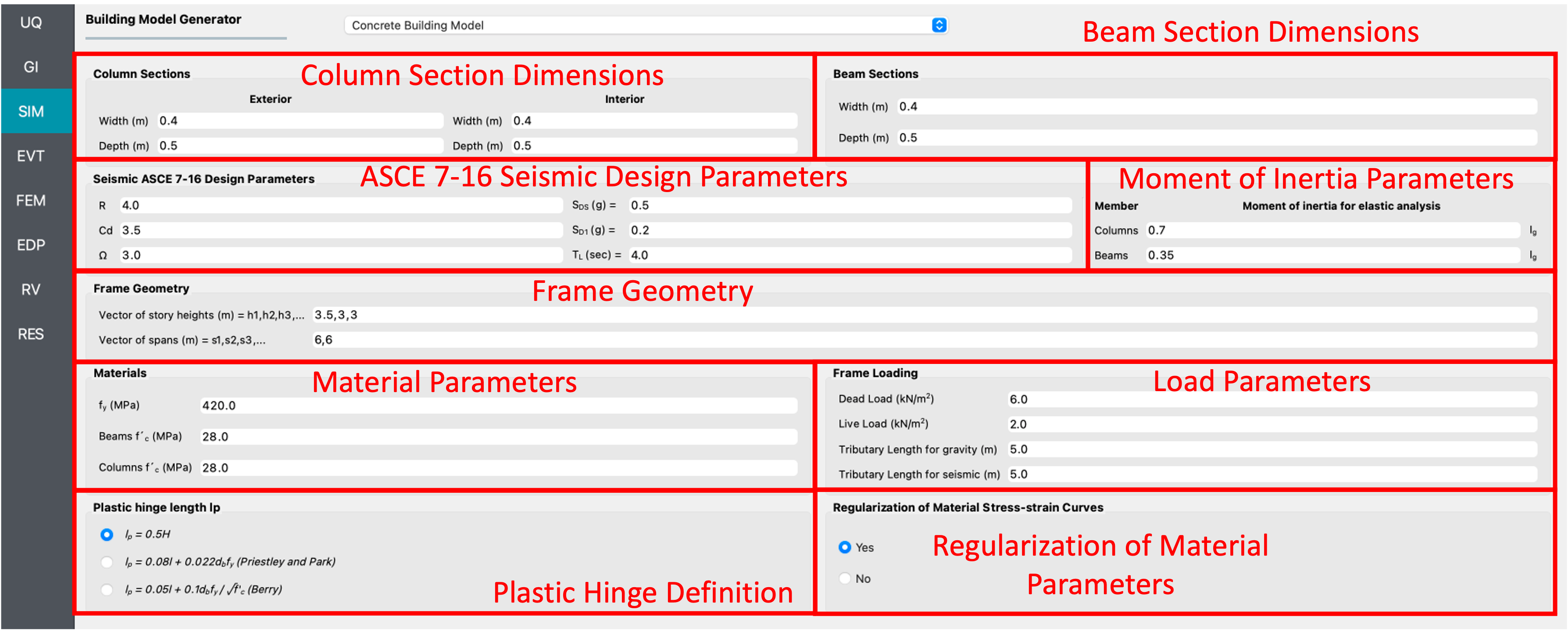
Fig. 2.3.4.1 Concrete Building Model.
2.3.5. Surrogate (GP)
In place of the physical simulation models, the Surrogate (Gaussian Process) model trained in EE-UQ can be imported.

Fig. 2.3.5.1 Loading a surrogate model
When users select the Surrogate (GP) option, they are requested to provide Surrogate info file (.json) that contains the information about the surrogate model. The surrogate info file can be created by training a surrogate model through EE-UQ.
GP output can be set as either the median prediction or a random sample generated from the normal distribution (or lognormal distribution if the user used log-transform when training) with the predictive median and variance. NOTE: the random generator does not account for the Gaussian process correlation, and each realization of EDP given the surrogate input parameters is independent of each other.
For the users who are interested in the advanced options please refer to the quoFEM user manual.
Note
Once the surrogate model is imported, the RV tab will be auto-populated and EDP names will be displayed under the surrogate model file path. The users can populate EDP tab using the names. The users may not add or remove EDPs.
Important
The user who selected “surrogate (GP)” option in the SIM tab must select “None” in FEM and EDP tabs. Otherwise, EE-UQ will give an error.
2.3.6. MDOF-LU Building Model
The MDOF-LU building modeling application creates a hysteretic, multi-degree of freedom (MDOF) model based on the Lu method. As seen in Fig. 2.3.6.1, the following inputs are required:

Fig. 2.3.6.1 MDOF-LU Building model input panel.
Hazus Data File: The path to a file that contains the ruleset that maps the design code-level & structural types to various structural parameters.
Hereis an example file, where the columns are in the order ofColumn names of HazusData.txt (click)
Table 2.3.6.1 Column names of HazusData.txt (showing the first 10 rows for high-code) id
str type
min #story
max #story
height
Sy
eta
C
gamma
eta_soft
alpha
beta
a_k
omega
damage1
damage2
damage3
damage4
T1
T2
hos
damp
1
W1
1
50
18.4547
0.4
0.0870354
1000
0.8
-0.001
3
1
0.1
0.2
0.004
0.012
0.04
0.1
0.35
0.33333
4.27
0.1
2
W2
1
50
56.243
0.4
0.0794118
1000
0.6
-0.001
2.5
1
0.1
0.2
0.004
0.012
0.04
0.1
0.2
0.33333
3.66
0.1
3
S1L
1
3
38.7247
0.25
0.0865974
1000
1
-0.001
3
1
0
0.2
0.006
0.012
0.03
0.08
0.25
0.33333
3.66
0.05
4
S1M
4
7
51.7562
0.156
0.133734
1000
1
-0.001
3
1
0
0.2
0.004
0.008
0.02
0.0533
0.216
0.33333
3.66
0.05
5
S1H
8
50
62.9659
0.098
0.181032
1000
1
-0.001
3
1
0
0.2
0.003
0.006
0.015
0.04
0.17
0.33333
3.66
0.05
6
S2L
1
3
56.243
0.4
0.0670927
1000
0.5
-0.001
2
1
0
0.2
0.005
0.01
0.03
0.08
0.2
0.33333
3.66
0.05
7
S2M
4
7
75.8694
0.333
0.103936
1000
0.5
-0.001
2
1
0
0.2
0.0033
0.0067
0.02
0.0533
0.172
0.33333
3.66
0.05
8
S2H
8
50
85.0452
0.254
0.142936
1000
0.5
-0.001
2
1
0
0.2
0.0025
0.005
0.015
0.04
0.136154
0.33333
3.66
0.05
9
S3
1
50
14.0607
0.4
0.0670927
1000
1
-0.001
2
1
0
0.2
0.004
0.008
0.024
0.07
0.4
0.33333
4.57
0.05
10
S4L
1
3
74.5959
0.32
0.0727412
1000
0.5
-0.001
2.25
1
0
0.2
0.004
0.008
0.024
0.07
0.175
0.33333
3.66
0.05
See Fig. 2.3.6.2 for the parameter definitions. Note that not all the parameters are being used.
Std deviation Stiffness: The standard deviation of lateral stiffness of the building model. The randomness will be applied by sampling a multiplication factor with the specified standard deviation and mean of 1. The factor is sampled only once per structure and will be applied to all stories.
Std deviation Damping: The standard deviation of the damping ratio of the building model. The randomness will be applied by sampling a multiplication factor with the specified standard deviation and mean of 1.
Default Story Height (optional): Used to set the mass node coordinates.
Once the analysis is done, the estimated structural parameters are written in SAM.json and the corresponding opensees model is written in example.tcl (with uniaxialMaterial Hysteretic material model) for the downstream analysis. Both files can be found in the local working directory.
Example of SAM.json (click)
{
    "Properties":
    {
        "dampingRatio": 0.09956333887469665,
        "uniaxialMaterials":
        [
            {
                "name": 1,
                "type": "shear",
                "K0": 61532397.052015901,
                "Sy": 2110124.6849974156,
                "eta": 0.087035399999999999,
                "C": 1000.0,
                "gamma": 0.80000000000000004,
                "alpha": 3.0,
                "beta": 1.0,
                "omega": 0.20000000000000001,
                "eta_soft": -0.001,
                "a_k": 0.10000000000000001
            },
            {
                "name": 2,
                "type": "shear",
                "K0": 61532397.052015901,
                "Sy": 1406749.7899982773,
                "eta": 0.087035399999999999,
                "C": 1000.0,
                "gamma": 0.80000000000000004,
                "alpha": 3.0,
                "beta": 1.0,
                "omega": 0.20000000000000001,
                "eta_soft": -0.001,
                "a_k": 0.10000000000000001
            }
        ]
    },
    "Geometry":
    {
        "nodes":
        [
            {
                "name": 1,
                "crd":
                [
                    0.0,
                    0.0,
                    0.0
                ],
                "ndf": 6,
                "constraints":
                [
                    1,
                    1,
                    1,
                    1,
                    1,
                    1
                ]
            },
            {
                "name": 2,
                "mass": 284190.39936000004,
                "crd":
                [
                    0.0,
                    0.0,
                    3.6000000000000001
                ],
                "ndf": 6,
                "constraints":
                [
                    0,
                    0,
                    1,
                    1,
                    1,
                    1
                ]
            },
            {
                "name": 3,
                "mass": 284190.39936000004,
                "crd":
                [
                    0.0,
                    0.0,
                    7.2000000000000002
                ],
                "ndf": 6,
                "constraints":
                [
                    0,
                    0,
                    1,
                    1,
                    1,
                    1
                ]
            }
        ],
        "elements":
        [
            {
                "name": 1,
                "type": "shear_beam2d",
                "uniaxial_material": 1,
                "nodes":
                [
                    1,
                    2
                ]
            },
            {
                "name": 2,
                "type": "shear_beam2d",
                "uniaxial_material": 2,
                "nodes":
                [
                    2,
                    3
                ]
            }
        ]
    },
    "NodeMapping":
    [
        {
            "cline": "response",
            "floor": "0",
            "node": 1
        },
        {
            "cline": "response",
            "floor": "1",
            "node": 2
        },
        {
            "cline": "response",
            "floor": "2",
            "node": 3
        }
    ],
    "units":
    {
        "force": "kN",
        "length": "m",
        "temperature": "C",
        "time": "sec"
    }
}
Example of opensees.tcl (click)
model BasicBuilder -ndm 3 -ndf 6
node 1 0 0 0
fix 1 1 1 1 1 1 1
node 2 0 0 3.6 -mass 284190 284190  0.0  0.0  0.0 2.8419e-05
fix 2 0 0 1 1 1 1
node 3 0 0 7.2 -mass 284190 284190  0.0  0.0  0.0 2.8419e-05
fix 3 0 0 1 1 1 1
uniaxialMaterial Hysteretic 1 2.11012e+06 0.0342929 6.33037e+06 0.822315 6.33037e+06 1 -2.11012e+06 -0.0342929 -6.33037e+06 -0.822315 -6.33037e+06 -1 0.8 0.8 0 0 0.1
uniaxialMaterial Hysteretic 2 1.40675e+06 0.0228619 4.22025e+06 0.54821 4.22025e+06 1 -1.40675e+06 -0.0228619 -4.22025e+06 -0.54821 -4.22025e+06 -1 0.8 0.8 0 0 0.1
element zeroLength 1 1 2 -mat 1 1 -dir 1 2
element zeroLength 2 2 3 -mat 2 2 -dir 1 2
loadConst -time 0.0
#timeSeries Path 101 -dt 0.005 -factor [expr 1 * 1 * 1 ] -values { -1.46509e-05 8.24738e-06 -2.26001e-05 1.46955e-05 -2.63045e-05 ..... -3.42224e-05  }
#timeSeries Path 102 -dt 0.005 -factor [expr 1 * 1 * 1 ] -values { 7.15223e-06 -2.4271e-05 1.94678e-05 -3.62861e-05 2.96503e-05 ...... -0.000675427  }
pattern UniformExcitation 101 1 -fact 1 -accel 101
set numStep 60000
set dt 0.005
pattern UniformExcitation 102 2 -fact 1 -accel 102
set numStep 60000
set dt 0.005
set numberOfStories 2
recorder EnvelopeNode -file 1-AIM.json0.max_abs_acceleration.response.0.out -timeSeries 101 102  -node 1 -dof 1 2  accel
recorder EnvelopeNode -file 1-AIM.json0.max_abs_acceleration.response.1.out -timeSeries 101 102  -node 2 -dof 1 2  accel
recorder EnvelopeNode -file 1-AIM.json0.max_rel_disp.response.1.out -node 2 -dof 1 2  disp
recorder EnvelopeDrift -file 1-AIM.json0.max_drift.response.0.1.1.out -iNode 1 -jNode 2 -dof 1 -perpDirn 3
recorder EnvelopeDrift -file 1-AIM.json0.max_drift.response.0.1.2.out -iNode 1 -jNode 2 -dof 2 -perpDirn 3
recorder EnvelopeNode -file 1-AIM.json0.max_abs_acceleration.response.2.out -timeSeries 101 102  -node 3 -dof 1 2  accel
recorder EnvelopeNode -file 1-AIM.json0.max_rel_disp.response.2.out -node 3 -dof 1 2  disp
recorder EnvelopeDrift -file 1-AIM.json0.max_drift.response.1.2.1.out -iNode 2 -jNode 3 -dof 1 -perpDirn 3
recorder EnvelopeDrift -file 1-AIM.json0.max_drift.response.1.2.2.out -iNode 2 -jNode 3 -dof 2 -perpDirn 3
recorder EnvelopeDrift -file 1-AIM.json0.max_roof_drift.response.0.2.1.out -iNode 1 -jNode 3 -dof 1 -perpDirn 3
recorder EnvelopeDrift -file 1-AIM.json0.max_roof_drift.response.0.2.2.out -iNode 1 -jNode 3 -dof 2 -perpDirn 3

# Perform the analysis
numberer RCM
constraints Transformation
system Umfpack
integrator Newmark 0.5 0.25
test NormUnbalance 1.0e-2 10
algorithm Newton
analysis Transient -numSubLevels 2 -numSubSteps 10
set xDamp 0.0995633;
set lambdaN [eigen 3];
set lambdaI [lindex $lambdaN [expr 1 -1]];
set lambdaJ [lindex $lambdaN [expr 3 -1]];
set lambda1 [lindex $lambdaN 0]
set omega1 [expr pow($lambda1,0.5)];
set omegaI [expr pow($lambdaI,0.5)];
set omegaJ [expr pow($lambdaJ,0.5)];
set alphaM [expr $xDamp*(2*$omegaI*$omegaJ)/($omegaI+$omegaJ)];
set betaKinit [expr 0 *2.0*$xDamp/($omegaI+$omegaJ)];
set betaKcomm [expr 0 *2.0*$xDamp/($omegaI+$omegaJ)];
set betaKcurr [expr 1 *2.0*$xDamp/($omegaI+$omegaJ)];
rayleigh $alphaM $betaKcurr $betaKinit $betaKcomm;
set lambdaN [eigen 1];
set lambda1 [lindex $lambdaN 0]
set T1 [expr 2*3.14159/$lambda1]
set dTana [expr $T1/20.]
if {$dt < $dTana} {set dTana $dt}
analyze [expr int($numStep*$dt/$dTana)] $dTana
remove recorders
where the keys of SAM.json are defined as follows:
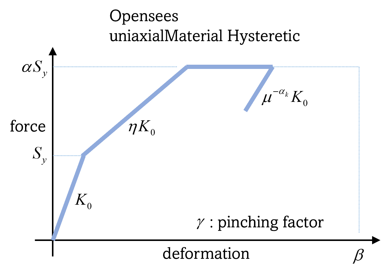
Fig. 2.3.6.2 MDOF-LU Building model.
Note
When the MDOF-LU building modeling application is employed, the OpenSees simulation application should be used for analysis in the ANA: Asset Analysis input panel.
Lu, X., McKenna, F., Cheng, Q., Xu, Z., Zeng, X., & Mahin, S. A. (2020). An open-source framework for regional earthquake loss estimation using the city-scale nonlinear time history analysis. Earthquake Spectra, 36(2), 806-831.
2.3.7. Multiple Models
The Multiple Models structural modeling application allows users to define multiple structural models for use in their analysis. The Add and Remove buttons allow users to control the number of models they want to use in the analysis.
By adding a model, a new tab is created in the SIM panel where users can choose one of the structural modeling applications described in the sections above and provide the inputs necessary to create the model. Users also need to specify their belief about the credibility of the model in the tab corresponding to that model. The beliefs are expressed as non-negative numerical values. The belief value for each model is defined relative to the other models, and the beliefs do not need to sum to 1.
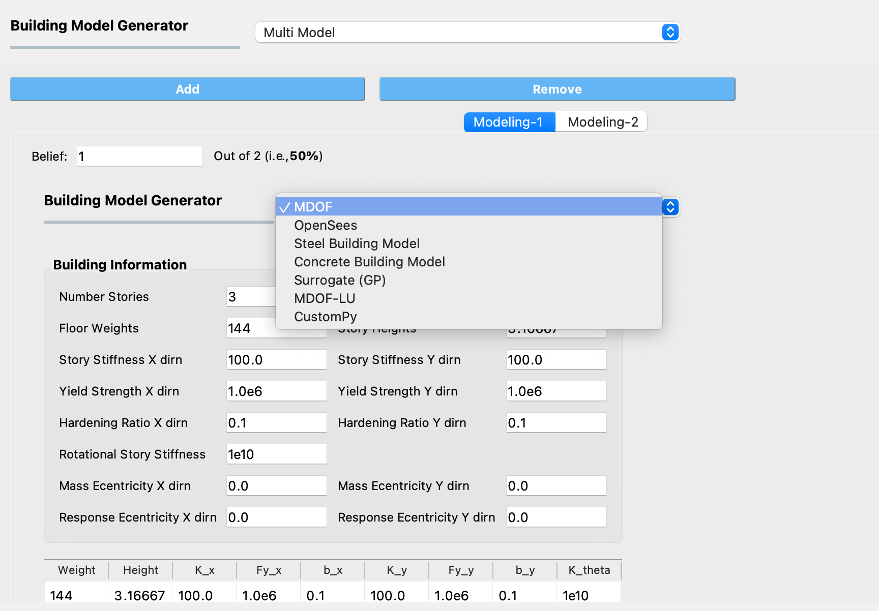
Fig. 2.3.7.1 Selecting a structural modeling application within a Multiple Models SIM Application
Note
If a Multiple Models application is selected, at least 2 models must be defined.
Note
If the “Multi-fidelity Monte Carlo (MFMC)” option was selected in the UQ tab, the belief values will be ignored. The premise of MFMC is that the high-fidelity model response always provides the best response, therefore, the conception of belief does not apply.