2.7.1.5. Outputs

This tab controls the types of output data generated throughout the calculation (Fig. 2.7.1.5.1). These outputs are stored in the local jobs directory (see its location under Preferences).

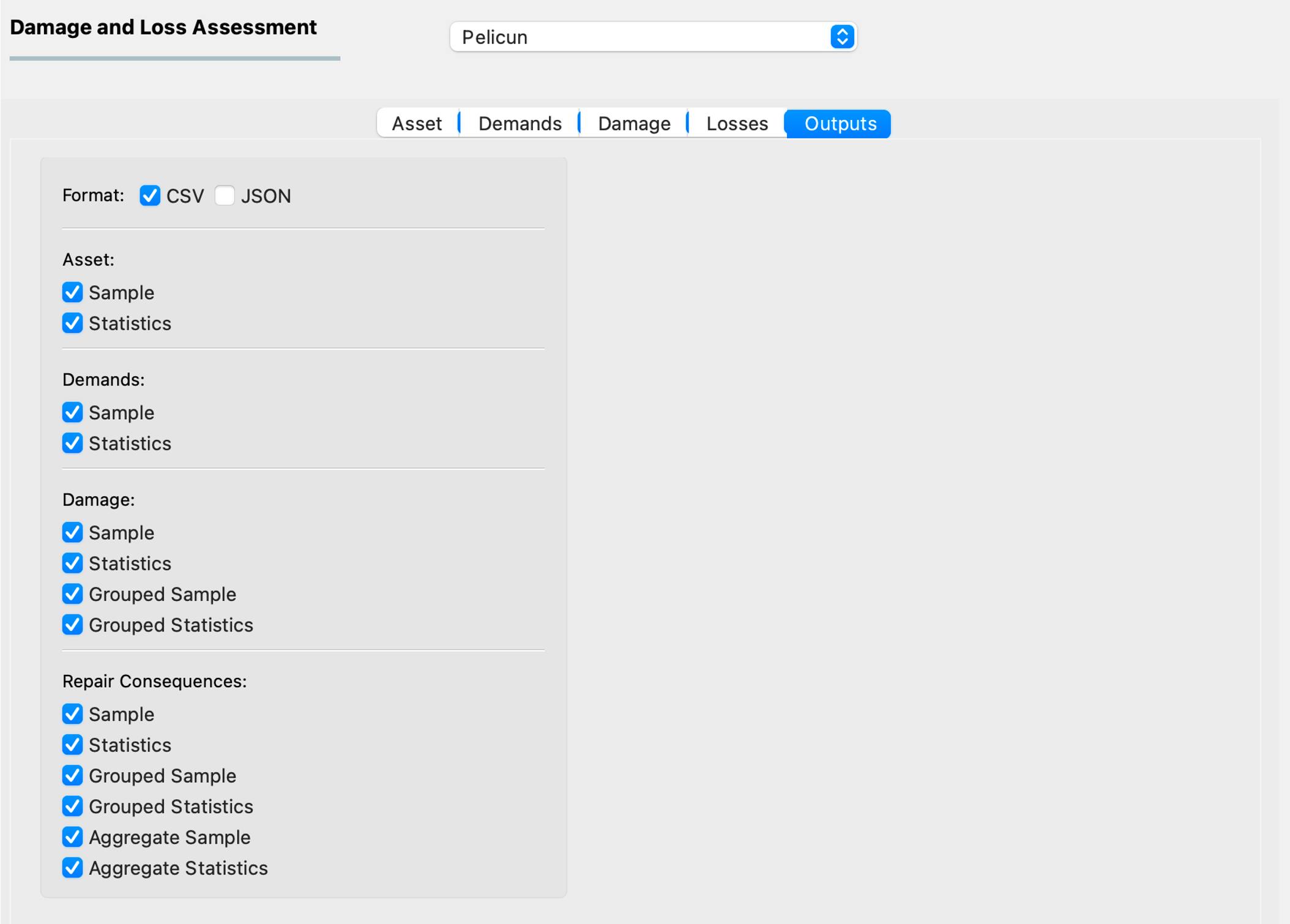
Fig. 2.7.1.5.1 The settings for calculation outputs.

All outputs can be saved in either CSV or JSON format. The descriptions below focus on the tabular organization of the CSV format. Each JSON output is generated by using the column labels in the header of the corresponding CSV table as a first-level list of keys. The value assigned to each of these keys is the contents of the corresponding column as an array or dictionary. Arrays are used for files that store a sample, while dictionaries are used for files of statistics where the index of the table needs to be preserved. The sample files are automatically zipped to reduce their size.The following sections introduce each output type with the corresponding table headers and structure.

Every output has a sample and a statistics version. The sample file provides information on every individual realization (identified by the index of the table) of the probabilistic calculation. The statistics file provides summary statistics based on the data in the sample. The following statistics are available:

sample size

The count row provides the number of valid values in each column of the sample file. This might be fewer than the total number of realizations in the damage and loss assessment if certain outputs are conditioned on other events, such as collapse and non-collapse cases.

mean

The mean row provides the mean of each column in the sample file.

standard deviation

The std row provides the standard deviation of each column in the sample file. The number of degrees of freedom is set to N-1, where N is the sample size. This yields an unbiased estimate of the variance and a corrected sample standard deviation. Note that while this is a much better estimate than using N degrees of freedom, it is still not an unbiased one. For the typical sample sizes of N>100, the bias in this statistic is negligible.

median

The 50% row provides the 50th percentile, also known as the median, of each column of the sample file.

log standard deviation

The log_std row provides the standard deviation (with the same N-1 degrees of freedom for bias-correction) in logarithmic space for each column in the sample file. When a column in the sample includes zero or negative values, the log standard deviation for that column is undefined and left empty.

extreme values

The min and max rows provide the minimum and maximum values of each column in the sample file.

mean ± 1,2,3 standard deviations

Assuming a normal distribution, the following percentiles are -3, -2, -1, 1, 2, 3 standard deviations from the mean: 0.10%, 2.30%, 15.90%, 84.10%, 97.70%, 99.90%. Each of these rows provides percentiles for each column in the sample file.

10th and 90th percentiles

The 10% and 90% rows provide the 10th and the 90th percentiles for each column in the sample file. The 90th percentile is often used as the so-called probable maximum value and its opposite, the 10th percentile is considered a lower bound in several applications.

Asset

The CMP_sample.csv (Fig. 2.7.1.5.2) and CMP_stats.csv (Fig. 2.7.1.5.3) files provide information on the types and quantities of damageable components assigned to the asset. Each column in the table corresponds to a component at a given location and direction. The label of each column is structured as componentID-location-direction. The quantities are measured in the units specified during component assignment.

The component quantity sample file is helpful in assessments with probabilistic component quantities. When the component quantities are deterministic, the sample file will contain identical rows. The statistics file provides a more concise option if you want to preserve deterministic component quantity assignments.

Fig. 2.7.1.5.2 The CMP_sample.csv output file with the component quantity sample.

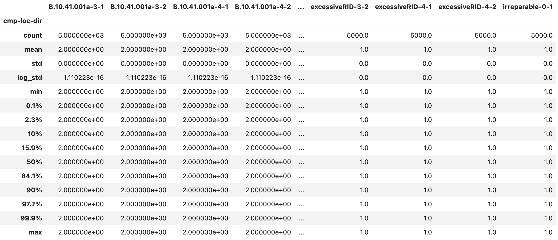
Fig. 2.7.1.5.3 The CMP_stats.csv output file with the component quantity statistics.

Demands

The DEM_sample.csv (Fig. 2.7.1.5.4) and DEM_stats.csv (Fig. 2.7.1.5.5) files provide information on the types and sizes of demands applied to the asset. Each column in the table corresponds to a demand type at a given location and direction. The label of each column is structured as event-demand-location-direction. Demands are measured in the units specified during demand assignment. The lbl-dldb_demands section provides more information on demand labels and units.

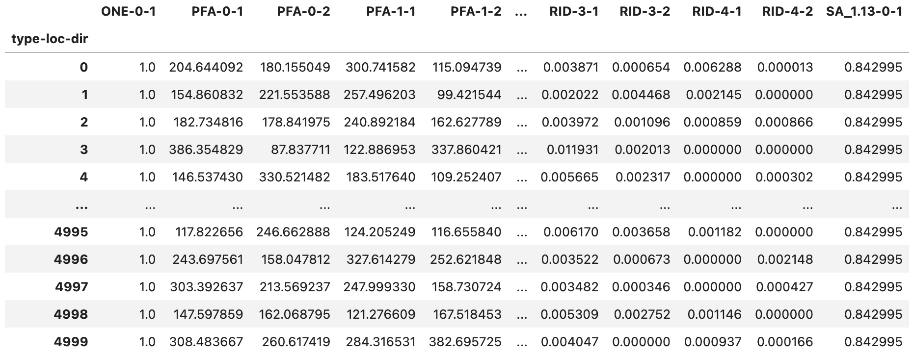
Fig. 2.7.1.5.4 The DEM_sample.csv output file with the demand sample.

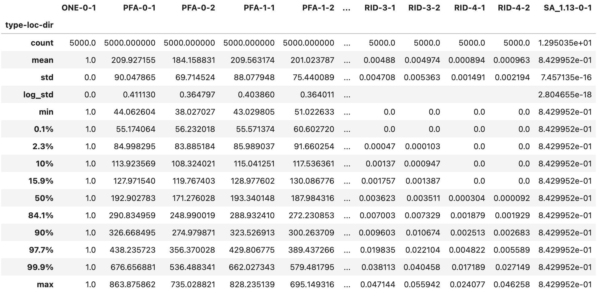
Fig. 2.7.1.5.5 The DEM_stats.csv output file with the demand statistics.

Damage

The DMG_sample.csv (Fig. 2.7.1.5.6) and DMG_stats.csv (Fig. 2.7.1.5.7) files provide information on the quantity of components in each damage state in each location and direction. The label of each column is structured as componentID-location-direction-ds, where ds stands for damage state. Damaged component quantities are provided in the units specified during component assignment.

The ds=0 option is included in the output and it provides the quantity of undamaged components for convenience. For the sake of efficiency, if a component type at a given location-direction is not damaged in any of the realizations, it is not included in the output. Furthermore, damage states that are never triggered (i.e., columns that would have all zero quantities) are also removed from the output. This behavior is controlled by optional settings in Pelicun that keep the output file sizes manageable. Let us know if there is interest in outputs with a comprehensive list of component-location-direction-ds; we can make such options available through the PBE app.

Note

Some of the rows can be almost entirely empty if the assessment includes global vulnerabilities, such as collapse, that render other component damages undefined (see Damage Processes under Damage Models). In such cases, the columns corresponding to the collapse component will identify the realizations (i.e., rows) where collapse was observed and other damages were not evaluated.

In the figures below, for example, realizations 4995, 4998, and 4999 are collapses and we see no damage quantities for other components. In the statistics file, we see that there are 4134 realizations with valid damage quantities for the first component. That yields a 4134/5000 = 82.68% probability of non-collapse outcomes.

Collapse is used here to demonstrate a common example that can lead to undefined damage quantities. Complex damage processes can introduce sophisticated interdependencies in the damage simulation that can yield similarly undefined damages for a subset of components.

Fig. 2.7.1.5.6 The DMG_sample.csv output file with the damaged component quantity sample.

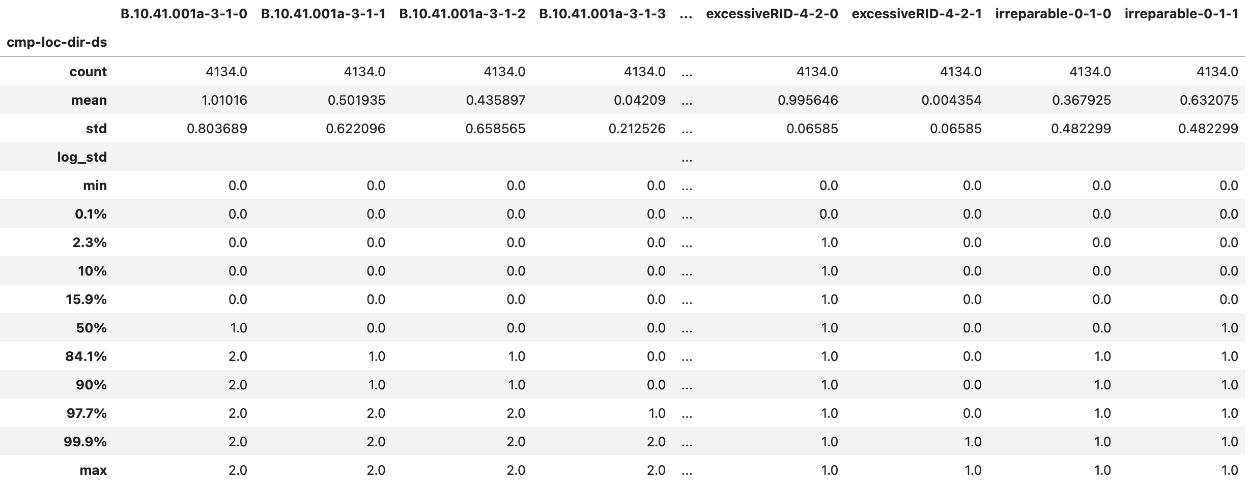
Fig. 2.7.1.5.7 The DMG_stats.csv output file with the damaged component quantity statistics.

Two additional output files provide grouped component damage information. The DMG_grp.csv (Fig. 2.7.1.5.8) aggregates damage quantities from the DMG_sample.csv across locations and directions. In other words, it provides the total quantity of components in each damage state across the entire asset. Its column labels are structured as componentID-ds. The DMG_grp_stats.csv (Fig. 2.7.1.5.9) provides statistics for the grouped damage sample.

Fig. 2.7.1.5.8 The DMG_grp.csv output file with the aggregate damaged component quantity sample.

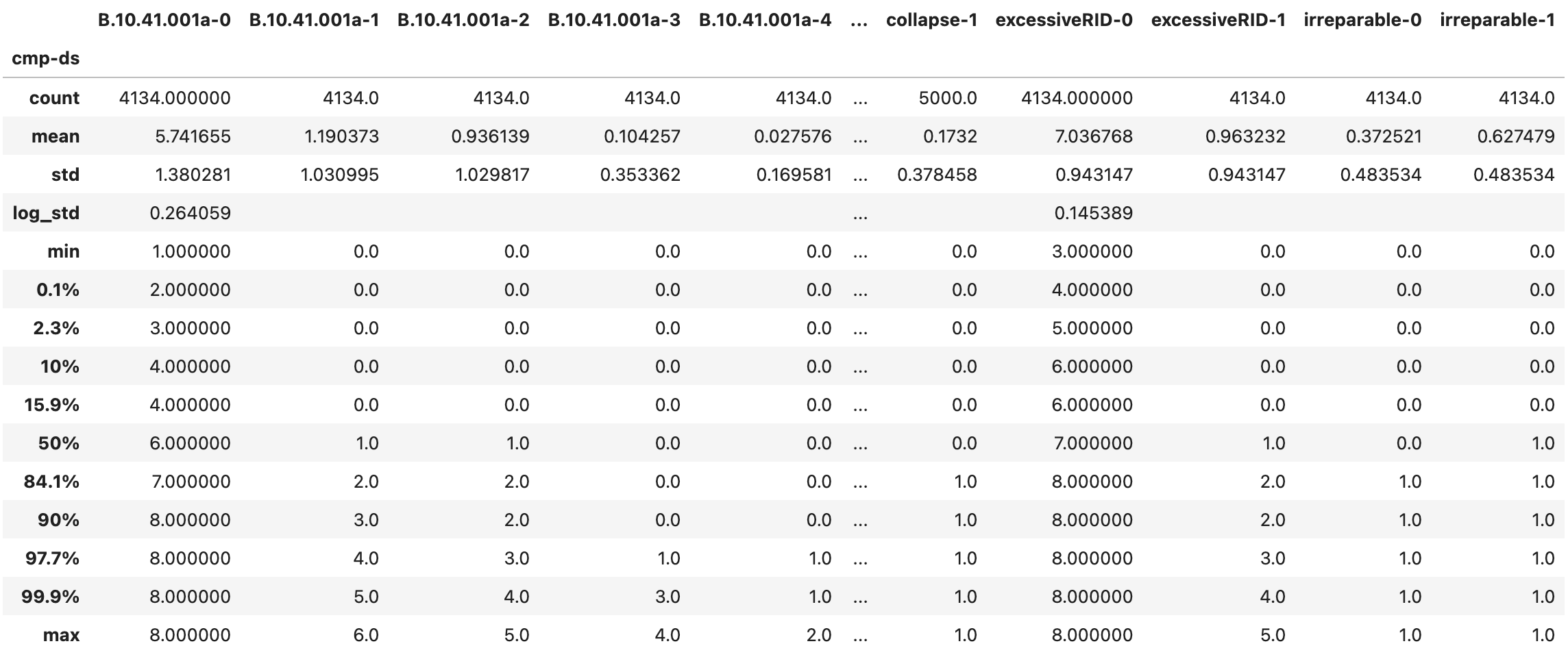
Fig. 2.7.1.5.9 The DMG_grp_stats.csv output file with the aggregate damaged component quantity statistics.

Repair Consequences

The DV_bldg_repair_sample.csv (Fig. 2.7.1.5.10) and DV_bldg_repair_stats.csv (Fig. 2.7.1.5.11) files provide detailed information on the repair consequences. The label of each column is structured as consequenceType-lossComponentID-damageComponentID-ds-location-direction, where consequenceType identifies the repair consequence (Carbon, Cost, Energy, and Time are currently supported); damageComponentID identifies which component’s damage resulted in the consequence; and lossComponentID identifies the component used to model the consequences. Consequence values are currently provided in the default units of the loss components.

The ds=0 option is included in the output and it provides the quantity of undamaged components for convenience. For the sake of efficiency, if a component type at a given location-direction is not damaged in any of the realizations, it is not included in the output. Furthermore, damage states that are never triggered (i.e., columns that would have all zero quantities) are also removed from the output. This behavior is controlled by optional settings in Pelicun that keep the output file sizes manageable. Let us know if there is interest in outputs with a comprehensive list of location-direction-ds; we can make such options available through the PBE app.

Note

Unlike damage information, the repair consequences are always available, that is, they cannot be undefined or missing in the output. When a component unit’s damage is undefined in a realization, for example, because the building collapsed in that realization, the component’s repair consequences will be zero. Hence, we can interpret the consequence outputs as “the contribution of each component unit to the total repair consequences”. If the building needs to be replaced, we do not count individual component contributions, hence those are zero in the output.

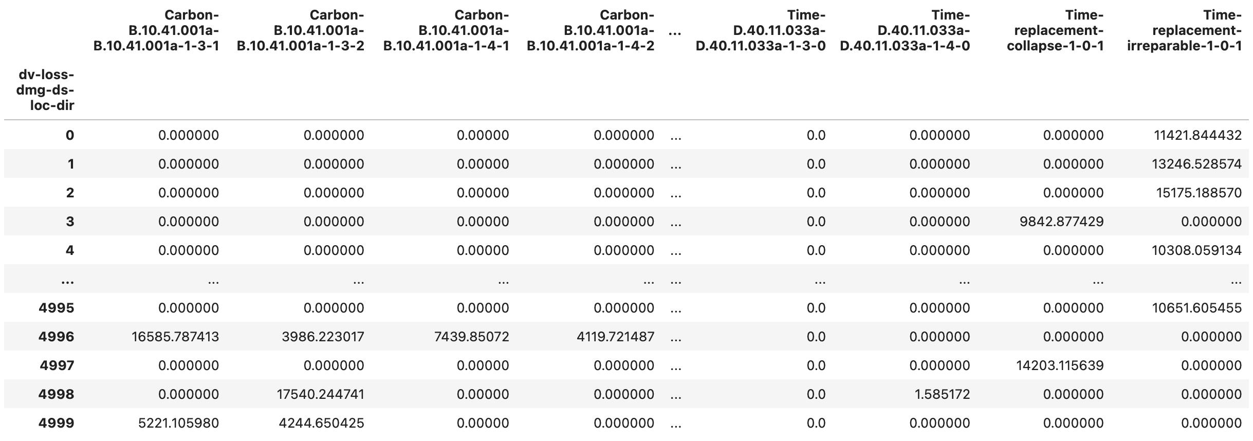
Fig. 2.7.1.5.10 The DV_bldg_repair_sample.csv output file with the repair consequence sample for each component.

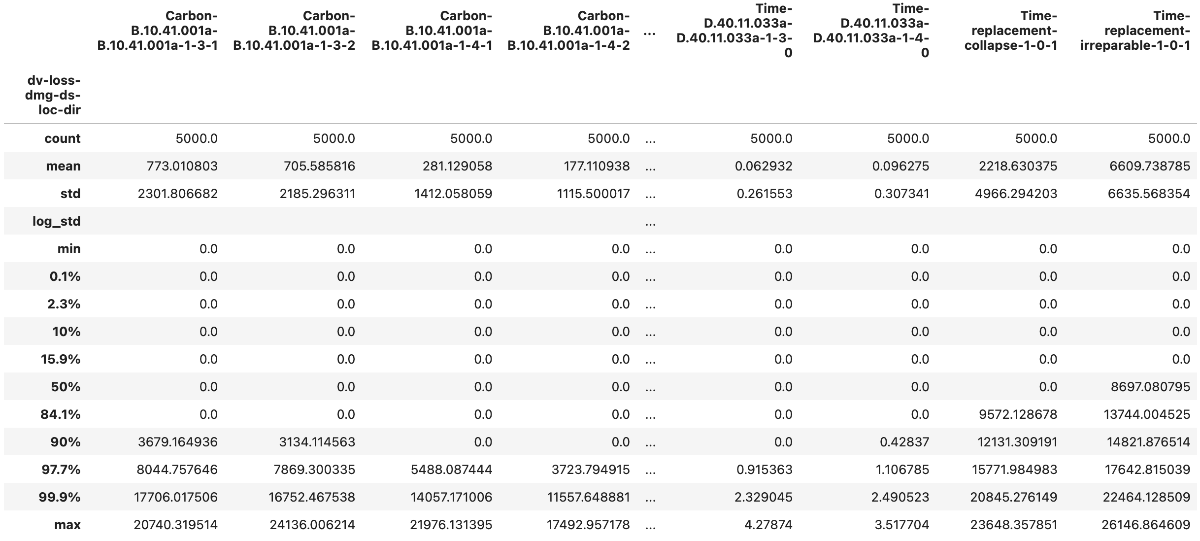
Fig. 2.7.1.5.11 The DV_bldg_repair_stats.csv output file with the repair consequence statistics for each component.

Two additional output files provide grouped component repair consequence information. The DV_bldg_repair_grp.csv (Fig. 2.7.1.5.12) aggregates consequences from the DV_bldg_repair_sample.csv across locations and directions. In other words, it provides the total repair consequence for each component type across the entire asset. Its column labels are structured as consequenceType-lossComponentID-damageComponentID. The DV_bldg_repair_grp_stats.csv (Fig. 2.7.1.5.13) provides statistics for the grouped damage sample.

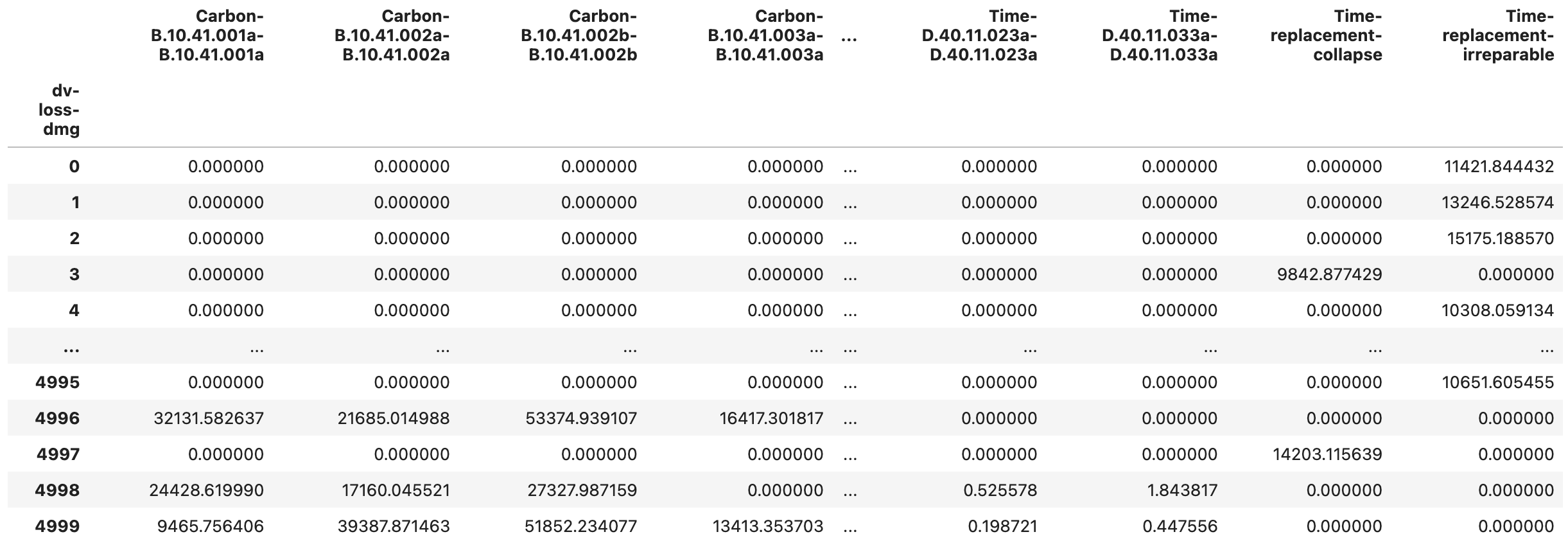
Fig. 2.7.1.5.12 The DV_bldg_repair_grp.csv output file with the grouped repair consequence sample for each component type.

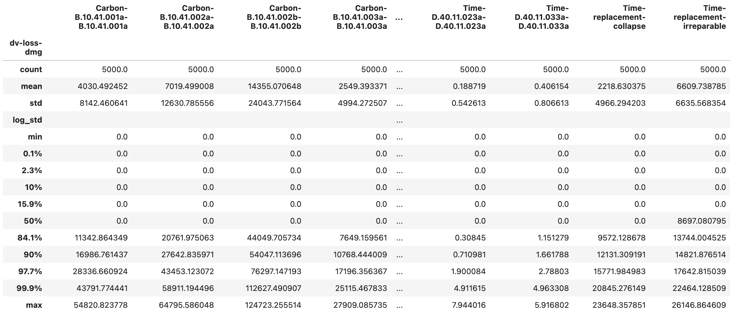
Fig. 2.7.1.5.13 The DV_bldg_repair_grp_stats.csv output file with the grouped repair consequence statistics for each component.

Finally, the aggregate sample and statistics files provide a high-level overview of the repair consequences by aggregating them across all components within the asset. Repair costs and embodied carbon and energy are simply summed for each realization. Repair time is calculated using the two edge cases recommended in FEMA P58: The parallel sceanrio assumes that floors are repaired simultaneously, in parallel. The sequential sceanrio assumes that floors are repaired in a serial fashion, each floor’s repairs starting when the one below is finished. Neither of these assumptions are realistic, but they span the range of plausible repair times. If you seek more realisitc repair time estimates, we suggest using one of the functional recovery simulation methodologies that employ some form of repair sequencing. See the PRF: Recovery Performance Assessment section for the available methodologies and corresponding examples.

The DV_bldg_repair_agg.csv (Fig. 2.7.1.5.14) provides the aggregate consequences for every realization, while the DV_bldg_repair_agg_stats.csv (Fig. 2.7.1.5.15) provides statistics.

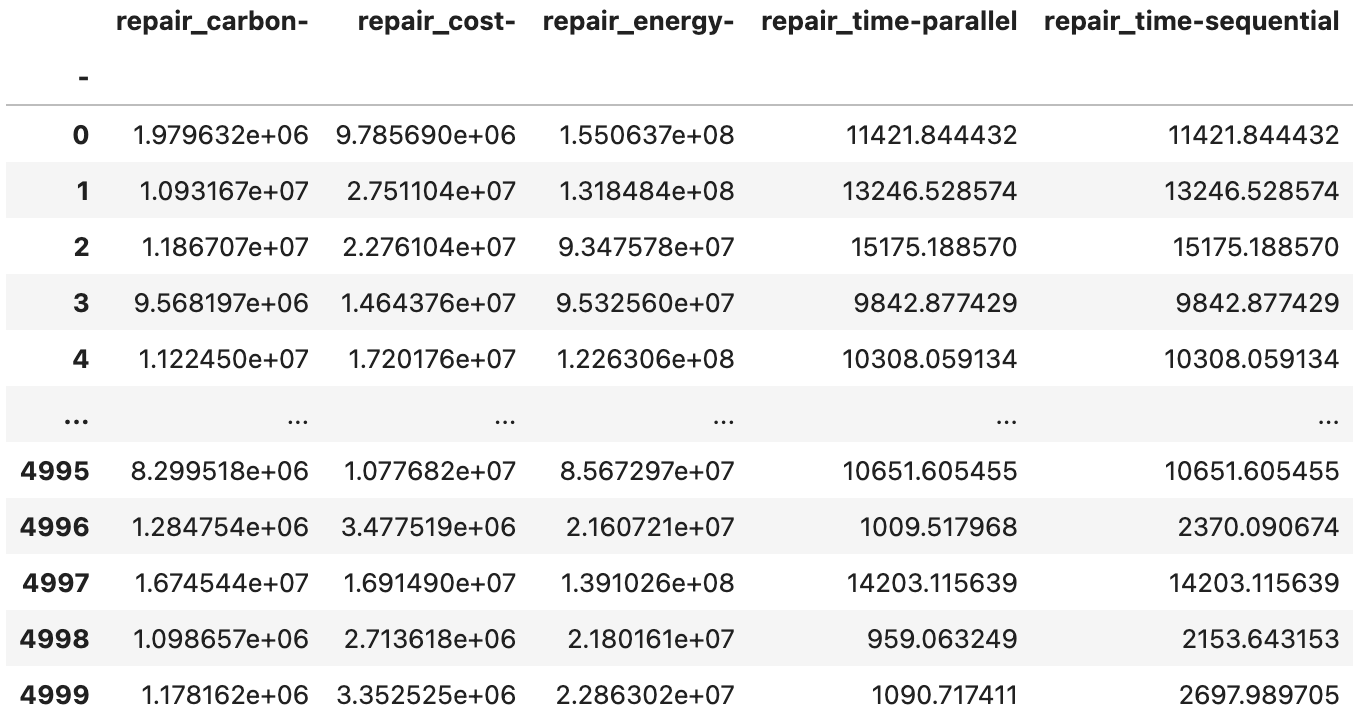
Fig. 2.7.1.5.14 The DV_bldg_repair_agg.csv output file with the aggregate repair consequence sample.

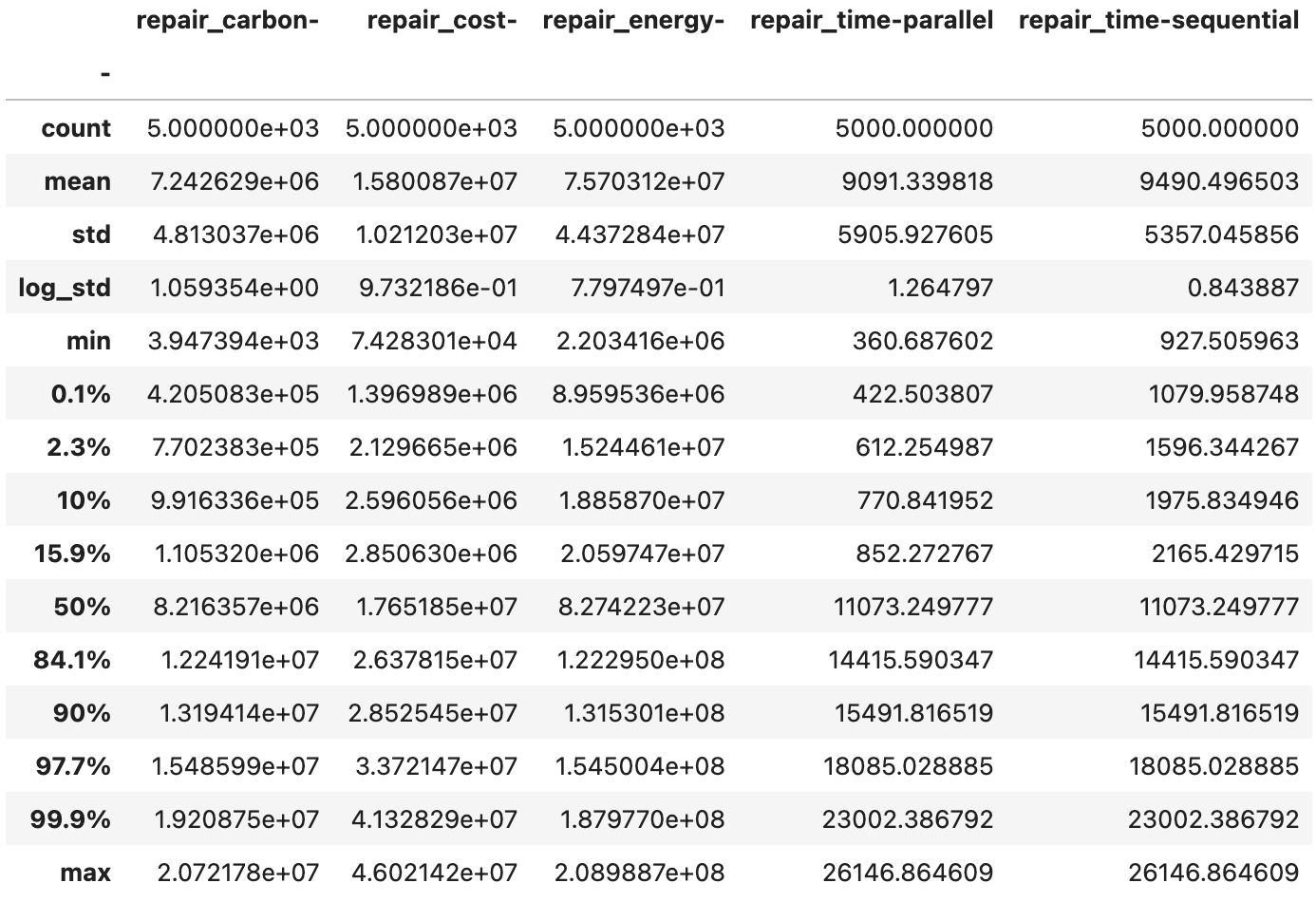
Fig. 2.7.1.5.15 The DV_bldg_repair_agg_stats.csv output file with the aggregate repair consequence statistics.