2.1.2.3. Reliability Analysis

Reliability methods are another class of probabilistic algorithms used for quantifying the effect of uncertainties in simulation input on response metrics of interest. These methods, unlike forward propagation analysis, provide the probability of response exceeding the user-provided threshold levels, i.e. given a set of uncertain input variables, it estimates the probability of system ‘failure’ defined as an excessive response. For reliability analysis, it is often more efficient to concentrate samples around the tail region of the response distributions, i.e. generating more events having low occurrence probability but high consequence, since often the number of samples required by naive sampling approach to resolve a low probability can be prohibitive.

Reliability methods can be split into local and global reliability methods and importance sampling-based methods, as elaborated in the following sections.

Problem Formulation

The probability of failure \(P_f\) is computed by the following integration:

(2.1.2.3.1)\[P_{f} = Pr \left[g(\mathbf{x}) \leq 0 \right] = \int_{g(\mathbf{x})\leq 0} f_\mathbf{X}(\mathbf{x})d\mathbf{x}\]

where \(f_\mathbf{X}(\mathbf{x})\) is the joint probability distribution of random variables (RVs), and \(g(\mathbf{x})\) is so-called the limit state function that indicates the system performance status: if \(g(\mathbf{x})\leq 0\) is true, then the system is regarded failed. For each quantity of interest (QoI), Dakota uses the following failure limit state function to compute \(P_{f}\):

(2.1.2.3.2)\[g(\mathbf{x}) = q_{tr} - q(\mathbf{x})\]

where \(q(\mathbf{x})\) is the computed value of QoI for given \(\mathbf{x}\) and \(q_{tr}\) is some response threshold value. So the failure probability here is equivalent to the probability of a response exceeding a certain threshold level. In the EE-UQ app, we use the following terminologies:

• Probability Level indicates \(P_{f}\)

• Response Level indicates \(q_{tr}\)

• Reliability Analysis computes \(P_{f}\) corresponding to \(q_{tr}\)

• Inverse Reliability Analysis computes \(q_{tr}\) corresponding to \(P_{f}\)

Local Reliability Methods

Local reliability methods introduce a first/second-order local approximation of the response or \(g(\mathbf{x})\) around either “Mean Value” or “Design point (also known as the most probable point, MPP)”. Each of these methods involves gradient-based local optimization. The local reliability methods can also be used for “inverse reliability problems” which aim to identify the unknown parameter (random variables) combination that produces prescribed probability levels. The user selects the local method using the pull-down menu.

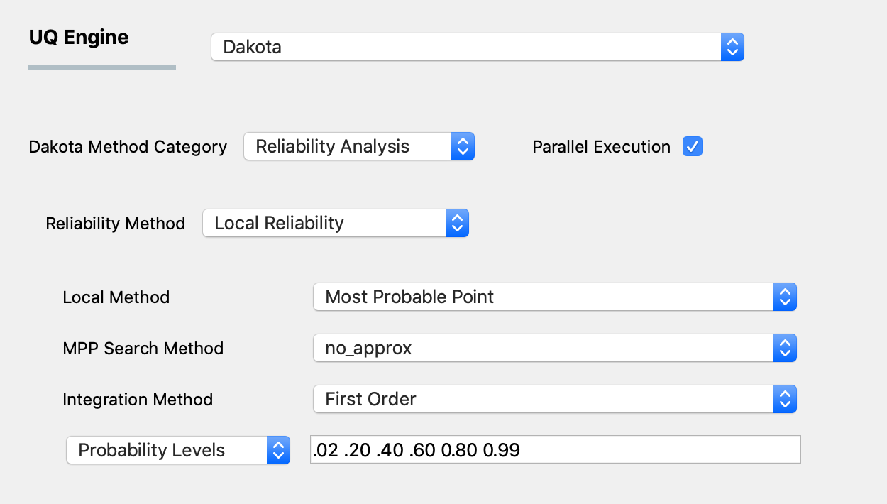
The default local reliability method is inverse reliability using the first-order reliability approximation (FORM) method. For the FORM method, the user provides the following inputs:

Fig. 2.1.2.3.1 Local reliability analysis using the MPP option.

1. The first input involves a selection of the MPP search method from the following options:

• no_approx: the MPP search on the original response functions without the use of any approximations. Combining this option with first-order and second-order integration approaches (see next section) results in the traditional first-order and second-order reliability methods (FORM and SORM).

• x_taylor_mean: a single Taylor series per response/probability level in x-space centered at the uncertain variable means. (Combined with a first-order approach, this is commonly known as the Advanced Mean Value (AMV) method, and combined with the second-order approach the method has been named AMV2:)

• u_taylor_mean: same as AMV/AMV2, except that the Taylor series is expanded in u-space, termed u-space AMV methods.

• x_traylor_mpp: an initial Taylor series approximation in x-space at the uncertain variable means, with iterative expansion updates at each MPP estimate until the MPP converges. The first-order option is commonly known as AMV+

• u_taylor_mpp: same as AMV+/AMV2+, except that the expansions are performed in u-space.

2. The second input involves the user selecting the integration approach for computing probabilities at the MPP. These can be selected to be first-order or second-order integration.

3. Finally the user selects either response levels (for forward reliability analysis) or probability level (for inverse reliability analysis) from a drop-down menu. The user then provides these levels in the line edit to the right of the pull-down menu.

Warning

Only a single quantity of interest (QoI) is allowed to be specified when using the most probable point searching. The Mean Value search method works for multiple QoIs.

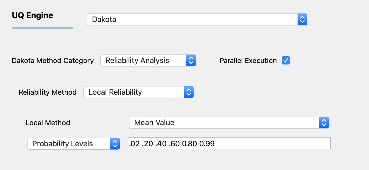
The second local reliability method available is the Mean Value method (also known as MVFOSM). It is the simplest and least-expensive reliability method because it estimates the response means, response standard deviations, and all response probability levels from a single evaluation of the response functions and their gradients at the uncertain variable means. This approximation can have acceptable accuracy when the response functions are nearly linear and their distributions are approximately Gaussian, but can have poor accuracy in other situations.

As shown in the figure below the user selects either to use response levels or probability levels. The user then inputs the levels.

Fig. 2.1.2.3.2 Local reliability analysis using the MVFOSM option.

Global Reliability Methods

Local reliability methods, while computationally efficient, do not always work. When confronted with a limit state function that is nonsmooth, local gradient-based optimizers may stall due to gradient inaccuracy and fail to converge to an MPP. Moreover, if the limit state is multimodal (multiple MPPs), then a gradient-based local method can, at best, locate only one local MPP solution. Finally, an approximation to the limit state at this MPP may fail to adequately capture the contour of a highly nonlinear limit state. Global reliability methods are designed to handle nonsmooth and multimodal failure surfaces. They do this by creating global approximations of \(g(\mathbf{x})\), say \(\tilde{g}(\mathbf{x})\), based on Gaussian process models. They accurately resolve a particular contour of a response function and then estimate probabilities using multimodal adaptive importance sampling.

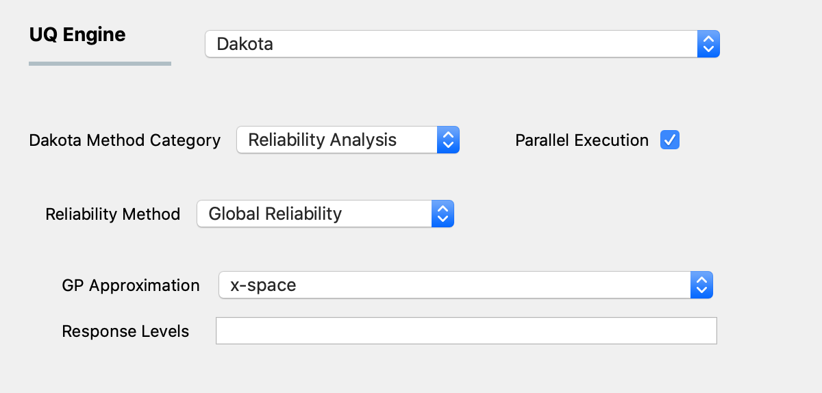
The user specifies if the Gaussian process is to be created in x-space (original) or u-space (transformed) [Read HERE for more about the transformation]. The user also specifies the response quantity levels (there is no option to define probability levels) and a seed.

Fig. 2.1.2.3.3 Global reliability analysis.

Warning

Only a single quantity of interest may be specified when using global reliability

Importance Sampling (IS)

For problems where one is interested in rare events rather than the whole distribution of output, such as earthquake or storm surge events, conventional sampling methods may require an excessively large number of simulations to obtain an accurate estimation of tail distribution. For such problems, importance sampling (IS) provides a bypass to conventional sampling methods (MCS or LHS), whereby an alternative sampling distribution is introduced around the tail part of the original distribution so that the generated samples have a better resolution at the domain of interest.

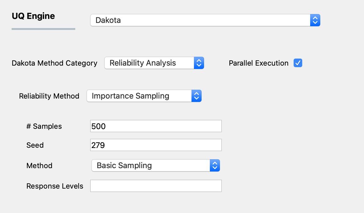
Fig. 2.1.2.3.4 shows the input panel for the IS scheme. Similar to MCS and LHS, IS requires both the number of samples to be executed and the corresponding seed for generating such random samples. In addition, the IS algorithm can be performed via three different approaches, as specified by the third input method:

1. Basic Sampling: A sampling density is constructed in the failure region based on an initial LHS sampling, followed by the generation of importance samples and weights and evaluation of the Cumulative Distribution Function.

2. Adaptive Sampling: The basic sampling procedure is repeated iteratively until a convergence in failure probability is achieved.

3. Multimodal Adaptive Sampling: A multimodal sampling density is constructed based on samples in the failure and the adaptive sampling procedure is used.

Fig. 2.1.2.3.4 Importance Sampling input panel.

Warning

Only a single quantity of interest may be specified when using importance sampling

For more information on each, please refer to the Dakota manual.