2.1.3.4. Probabilistic Learning on Manifolds (PLoM)

About PLoM

PLoM is an open-source Python package that implements the algorithm of Probabilistic Learning on Manifolds with and without constraints ([SoizeGhanem2016], [SoizeGhanem2020]) for generating realizations of a random vector in a finite Euclidean space that are statistically consistent with a given dataset of that vector.

PLoM functionality in SimCenter tools is built upon PLoM package (available under MIT license), an opensource Python package for Probabilistic Learning on Manifolds [ZhongGualGovindjee2021]. The package mainly consists of python modules and invokes a dynamic library for more efficiently computing the gradient of the potential, and can be imported and run on Linux, macOS, and Windows platforms.

Basic Model

The PLoM Model is a SimCenterUQ method to learn data structure and generate new realizations from a training dataset. It can be used for data sampling, dimension reduction, and surrogate modeling. Currently, there are two training data options: Import Data File and Sampling and Simulation.

Fig. 2.1.3.4.1 SimCenterUQ method: PLoM Model

Option 1: Import Data File

Under the Import Data File option, UQ Engine expects users to directly provide the training data matrices. For instance, users can upload tabulated data files for input variables and corresponding output responses, by using the Raw Data mode. Example input and output variables (PLoM_variables.csv and PLoM_responses.csv) are provided for demonstrating the format: (1) the first row describes the variable names, (2) the first variable name starts with “%”, and (3) data are tabulated from the second row.

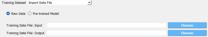
Fig. 2.1.3.4.2 User-provided raw data files for training dataset

New Sample Number Ratio is an integer defining the ratio of the new realization size and the input sample size. For instance, if the input file includes 100 data points, using a New Sample Number Ratio of 5 would produce 500 new realizations. In addition, if the New Sample Number Ratio is set to zero, then no new sample will be generated, however, the trained model can be saved.

Fig. 2.1.3.4.3 User-provided pre-trained model

The alternative mode to Raw Data is Pre-trained Model which allows users to upload the saved pre-trained model.

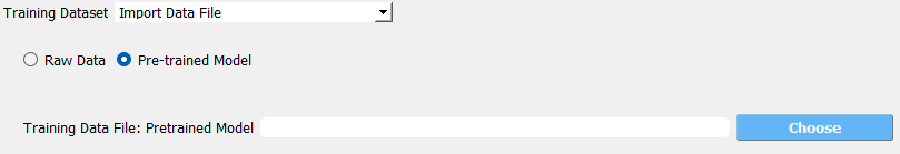
Fig. 2.1.3.4.4 User-provided pre-trained model

Option 2: Sampling and Simulation

Under the Sampling and Simulation option, UQ Engine will first invoke FEM applications (e.g., OpenSees) to run numerical simulations and generate the needed training dataset. So, instead of directly providing the training data, users are responsible for configuring the simulation model and analysis.

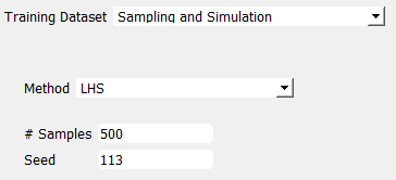
Fig. 2.1.3.4.5 User-provided pre-trained model

Advanced Options

Advanced users can configure more modeling parameters by checking Advanced Options checkbox.

General

• Log-space Transform: apply a logarithmic transformation to the data matrix

• Random Seed: enable replicating analysis

• PCA Tolerance: truncating eigenvalue model representation from principal component analysis

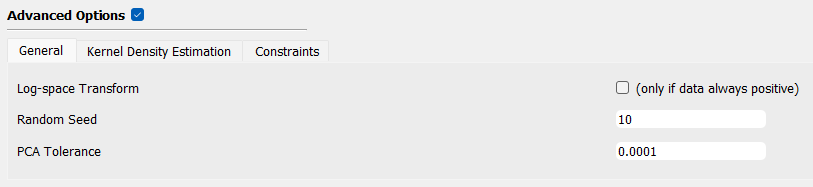
Fig. 2.1.3.4.6 PLoM advanced option: General

Kernel Density Estimation

• KDE Smooth Factor: smooth factor in kernel density base function

• Diffusion Maps: whether invokes diffusion maps

• Diff. Maps Tolerance: truncating ratio between the last considered eigenvalue and the first eigenvalue

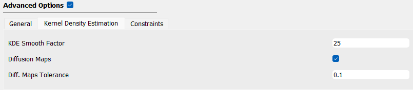
Fig. 2.1.3.4.7 PLoM advanced option: Kernel Density Estimation

Constraints

• Add constraints: whether applies constraints to the model

• Constraints file (.py): constraint file path

• Iteration Number: maximum number of iterations

• Iteration Tolerance: maximum tolerance in iteration

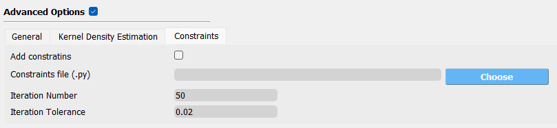
Fig. 2.1.3.4.8 PLoM advanced option: Constraints

User-Defined Variables

• None: no extra variables except for those defined in RV and EDP panel to be considered

• User-Defined: users can upload a script for computing the extra variables in the analysis

• Ground Motion Intensity: for earthquake simulation, the user can add various intensity measures as extra variables,

  for instance, Peak Ground Acceleration, Pseudo Spectral Acceleration at multiple periods

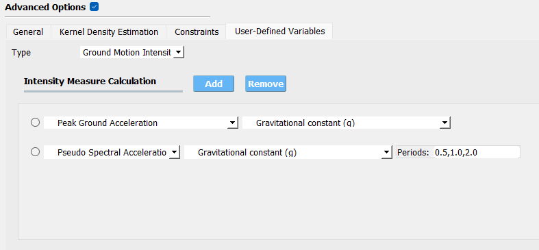
Fig. 2.1.3.4.9 PLoM advanced option: User-Defined Variables

Results and Postprocess

Once the training is completed, two plots will be generated in the RES panel for the PLoM training results:

• PCA: plots the curve of PCA representation error versus the PCA eigenvalues overlapped by the truncating PCA eigenvalue used in training.

• KDE: plots the curve of diffusion map eigenvalue by components overlapped by the truncating eigenvalue used in training

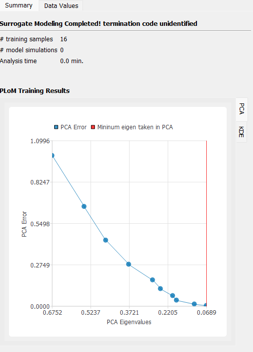
Fig. 2.1.3.4.10 PLoM training result plots: PCA

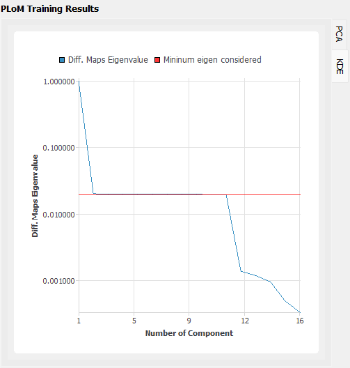
Fig. 2.1.3.4.11 PLoM training result plots: KDE

Users can also save the trained PLoM model by clicking on the Save PLoM Model at the bottom of the RES Summary page. The training data and model information will be saved as a .h5 data file to a user-defined directory, which can be loaded back for generating extra samples in the future (as described previously).

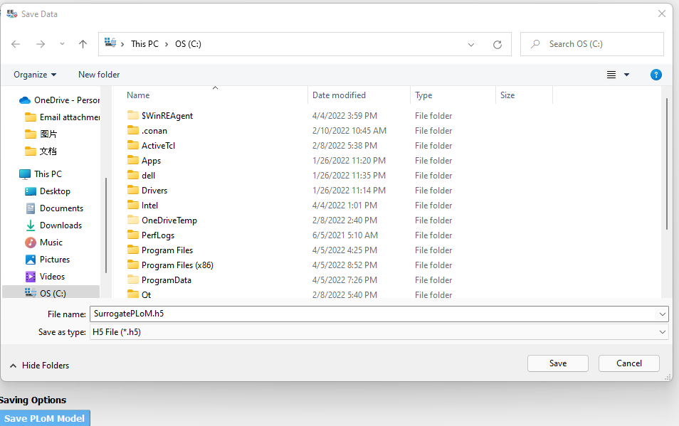
Fig. 2.1.3.4.12 Save PLoM model

The training data / new sample points can be visualized under the Data Values tab, and saved to a user-defined directory by clicking the Save Table or the ``Save Column Separately ``button on the top right corner.

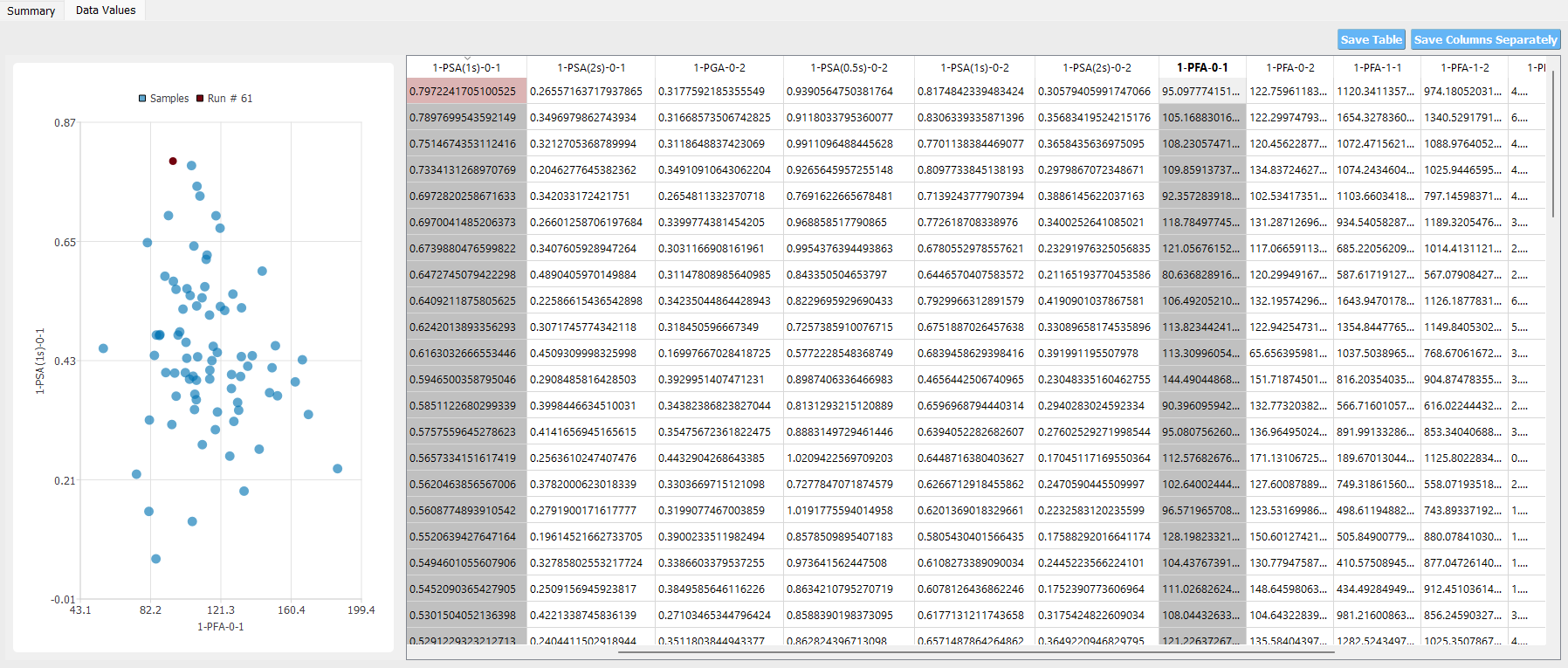
Fig. 2.1.3.4.13 Visualization of PLoM results

[SoizeGhanem2016]

Soize, C., & Ghanem, R. (2016). Data-driven probability concentration and sampling on manifold. Journal of Computational Physics, 321, 242-258.

[SoizeGhanem2020]

Soize, C., & Ghanem, R. (2020). Physics‐constrained non‐Gaussian probabilistic learning on manifolds. International Journal for Numerical Methods in Engineering, 121(1), 110-145.

[ZhongGualGovindjee2021]

Zhong, K., Gual, J., and Govindjee, S., PLoM python package v1.0, https://github.com/sanjayg0/PLoM (2021).