4. CFD Solvers
HydroUQ leverages the power of OlaFlow for the CFD solver. The
4.1. Turbulence models
During a coastal hazard and as the waves reach the coast, the boundary layer can be significantly complex. Further on, these waves can be broken / unbroken in-nature. When the flow is in the laminar regime, the fluid flow can be completely predictied by solving the Navier-Stokes equations. As the flow transitions to turbulence, as often seen in broken waves, oscillations appear in the flow. In this case, one needs to resolve the smallest eddies in the flow to order to accurately predict the flow fields and the response on the structure. As the Reynolds number increases, the flow field exhibits small eddies. At this point, the oscillations in spatial and temporal scales are computationally difficult to resolve for most of the practical cases.
When a direct numerical simulation (DNS) is employed, the Navier-Stokes equation is solved by resolving the whole range of spatial and temporal scales of the turbulence. This implies the resolution of the smallest dissipative scales (i.e. Kolmogorov microscales) up to the integral scale \(L\) associated with the motions containing the largest percentage of the kinetic energy.
Since DNS is computational expensive, the large eddy simulation was proposed by Joseph Smagorinsky in 1963. The idea of LES was to ignore the smaller length scales that are expensive to resolve. Using a low-pass filtering technique, the most expensively small-scale information is removed from the numerical solution.
The HydroUQ application presently does not support either DNS or LES simulations. At present, only Reynolds Averaged Navier-Stokes (RANS) simulations are supported by the HydroUQ. If you would like to use the DNS / LES, please leave a feature request on our message board.
RANS is based on the observation that the flow field contained a time-averaged state \((U)\) and small-local oscillations \((u')\). Additional transport equation(s) are introduced for the turbulence variables and solved with the velocity and pressure. Often these can be algebraic models that depend on parameters like the velocity of the flow, distance from the wall. These models help estimate the eddy viscosity due to turbulence and is added to the molecular viscosity of the fluid. The momentum that would be transferred by the small eddies is instead translated to a viscous transport. In general, the turbulence dissipation dominates over viscous dissipation everywhere, except in the viscous sublayer close to the solid walls. Wall models help resolve the right turbulence dissipation in these sublayers.
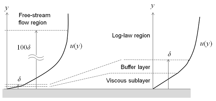
Fig. 4.1.1 Four regimes of the flow for a flow considered over a flat-plate
As shown in Fig. 4.1.1, the flow near a flat bottom can be divided into four regimes. The velocity of the fluid at the wall is nearly zero. Viscous effects domainate in a small thin layer above the wall. This is known as the viscous sublayer. Further away from the all is a transition region known as the buffer sublayer. Here, the turbulence stresses start to increase and dominate over the viscous stresses. Further away is the log-law region, where the flow is fully turbulent and the average velocity is related to the log of the distance to the wall. Even further away is the free-stream region. The thickness of the viscous and buffer sublayers are almost hundred times smaller than the log-law region. Thus, instead of resolving them, a wall model can be used that would assume an analytic solution for the flow in the viscous layer and thus reduce the computational costs. Such an approximation is reasonable for applications in geological flows.
There are several turbulence models available for usage. Among them, two models are made available for usage in the HydroUQ application. It is important to choose the right models for the application of interest.
4.2. Input file formats
The first important aspect is to understand the input file structure. The input file is in the form of three directories / folders, namely (a) time or 0 (b) system (c) constant
For more information, check out the educational app on OpenFOAM - i.e. CFD-Notebooks