6. Best Practices¶

6.1. Errors and uncertainties¶

There are several sources of errors that are often observed in CFD simulations. These include:

The model is described by the Navier-Stokes equations. The exact N-S equations are solved when Direct Numerical Simulations (DNS) are employed. However, when the RANS approach is involved, as in HydroUQ, this involves approximations that could lead to errors and uncertainties. Thus, selecting the correct parameters is paramount.
If the solution shows divergence, check the boundary conditions, grid, discretization, and convergence errors. Check whether the flow is steady or unsteady and the timestep used in this regard.

6.2. Froude number¶

One of the essential non-dimensional numbers that describe different flow regimes for open channel flow. It is a dimensionless quantity that is a ratio of the inertial and gravitational forces as \(Fr = \frac{V}{\sqrt{gD}}\). Here V is the water velocity, D is the hydraulic depth across the cross-sectional area of the flow, and g is the gravity.
It is important to calculate if the flow is sub-critical (Fr < 1) or critical (Fr = 1) or supercritical (Fr > 1). Critical flows are often unstable and set up standing waves between sub and supercritical flows.
It is necessary to consider both the Froude number and Reynolds number to determine separation effects like breaking waves.

6.3. Spatial discretization¶

Mesh checking is always essential. HydroUQ app performs a mesh check, and the log is available for review after the simulation is complete. It is much recommended to review this.
Mesh convergence study is critical to ensuring good and reliable results using CFD simulations. Thus, it is strongly recommended to estimate the error by refining the mesh, if possible.
Using a fine grid throughout may reduce the convergence rate. Instead, use grid adaptation or refine the mesh in areas of a large gradient to reduce computational cost. Use grid refinement where local details are required.
HydroUQ app has a basic mesher available that generates hex grids. For complex geometries, it is recommended to create hybrid grids using external meshing tools. Such grids can generally use prism layer grids in the boundary layer, tetrahedral cells in the core flow region, and hex grids.
It is recommended that the aspect ratio be below 5 but can be up to 10 inside the boundary layer. Ensure that the change in grid size is gradual, and the maximum variation in grid spacing should be less than 20%.

# Avoid highly skewed cells so that the angles between gridlines are orthogonal or near orthogonal. Angles with less than 40-degrees or greater than 140-degrees may lead to numerical instabilities or unsatisfactory results.

6.4. Temporal discretization¶

It is suggested to take a small timestep to start with so that it can be automatically increased to check the influence of timesteps on the results.
The timestep size should be decided based on the Courant-Friedrichs-Lewy (CFL) condition . Yet, it should also be small enough to capture any transient phenomena of interest.
Using the log files, ensure that the simulation has converged at each time step. For temporal accuracy, it is recommended to use a second-order accurate discretization scheme like Crank-Nicolson.

6.5. Boundary conditions¶

The EVT requires one to provide six boundary conditions for the six standard patches Entry, Exit, Right, Left, Bottom and Top.
If no boundary condition is specified for a particular patch, it is assumed to be type: empty by default. Presently, HydroUQ app only allows specification of the velocity and pressure boundary conditions. If you would like to specify other parameters, please write to us at Bugs & Feature Requests.
The inlet boundary condition should be used for patches where it has a weak influence on the downstream flow. Perform a sensitivity analysis on the inlet flow direction, magnitude, and profile. The exact inlet turbulence conditions are usually unknown. Thus, 1% turbulent intensity can be assumed for external flows.
The outlet boundary condition should be specified on the patch, which has a weak influence on the upstream flow. It is suggested to set the convective derivative normal to the outlet boundary face to be zero. However, for flow with strong pressure gradients, special non-reflecting boundary conditions would be required.
Ensure that the wall boundary conditions are specified for the solid walls.

6.6. SW-CFD domain sizes¶

Note that each degree of latitude is approximately 69 miles (111 km apart). At the Equator, the distance is 68.703 miles (110.567 km); at Tropic of Cancer and Capricorn, it is 68.94 miles (110.948 km), and at the poles, it is 69.94 miles (111.699 km).
60 minutes = 1 degree
For a 1-minute grid used in the SW-solver, this is approximately a 2 x 2 km grid (in terms of distances). This could still be a considerably large domain for the CFD simulation, depending on the topography and bathymetry.
If the simulation type is SW-CFD coupling, then there can be wave reflections. Such wave reflections can lead to unphysical fluid accumulation at the boundary.

6.7. Turbulence modeling¶

Compute the Reynolds number to determine if the flow is turbulent. Do not use turbulent models for laminar flows.
Estimate the y+ and the thickness of the first cell layer. The ideal distance of the first node from the wall \(\Delta y\) can be estimated to be

(6.7.1)¶\[\Delta y = L \cdot y^{+} \cdot \sqrt{74} \cdot {Re}_{L}^{-13/14}\]

where \(L\) is the characteristic length scale, \(y^{+}\) is the desired values, \({Re}_{L}\) is the Reynolds number. The non-dimensionalized velocity (\(u^{+}\)) and distance from the wall (\(y^{+}\)), the velocity profile of the boundary layers, takes on the form, as shown below by the red line in Fig. 6.7.1.

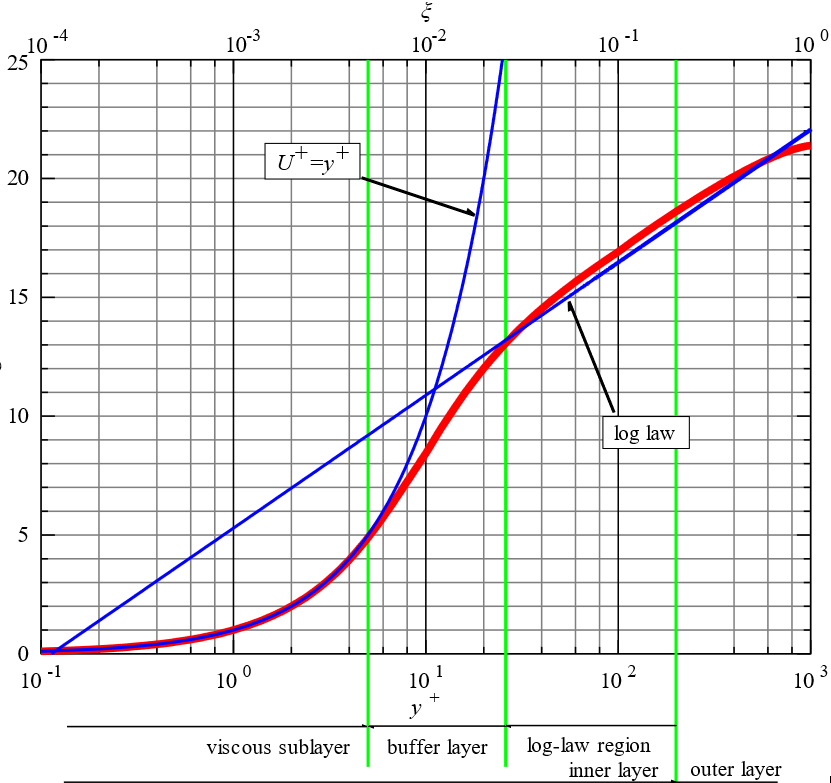
Fig. 6.7.1 The variation of non-dimensional velocity and distance¶

Various online calculators can be used to calculate the value of \(y^{+}\). Some examples of apps include: Google Play Store or Apple store .
If the flow is believed to be viscous, then the viscous sub-layers need to be resolved as shown in Fig. 6.7.2. When meshed correctly, a value of \(y^{+} \approx 1\) is desired. Alternatively, a wall model can be used bu having the first element in the region \(y^{+} > 30\). It is a good practice to avoid a \(y^{+}\) value between these values.

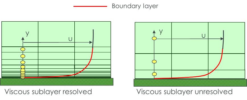
Fig. 6.7.2 Resolution of the viscous sub-layer¶
High Reynolds number flows (like aircraft, ships, etc.) will experience boundary layers that extend to several thousand \(y^{+}\) units. However, for flows with low Reynolds numbers, the upper limit can be as little as 100 \(y^{+}\) units. Thus, it is necessary to ensure that the first node does not fall outside this range.
HydroUQ app 1.0 supports \(k-\epsilon\) and \(k-\omega\) SST models. These are both good choices for general applications. The \(k-\epsilon\) model is very reliable and can often be used to get initial values for more sophisticated models.
The \(k-\epsilon\) model is inaccurate for flows with adverse pressure gradients. It does not allow integration of the conservation equations through the viscous sublayer where low Reynolds number corrections are recommended.
The \(k-\omega\) model is very sensitive to the freestream boundary conditions. However, it performs well for flows with variable pressure gradients.

6.8. User errors¶

Check for details in the geometry. Do not over-simplify the geometry without an understanding of the given problem.
Inaccurate use of boundary conditions, poor-quality grids are commonly observed user errors.
Ensure that the timestep sizes provided are reasonable.

6.9. Checking results¶

Check the overall mass balance.
Check whether the values and distribution of values of velocities, forces, and pressures are realistic.
Perform simple hand calculations in a smaller number of grids to check the orders of magnitude of variables. Alternatively, compare with similar problems or simplified versions of the same problem.
Perform a sensitivity analysis by changing the grid size, effects of boundary conditions, and turbulence models.