2. Finite Volume Method

Similar to other numerical methods, the Finite Volume Method (FVM) transforms a set of partial differential equations (PDE) into a system of linear algebraic equations. Using this method the governing PDE is satisfied over finite-sized control volumes, rather than at points as in other PDE discretization techniques. The Finite Difference Method (FDM) and the Finite Element Method (FEM) have been traditionally used to operate on PDEs. However, simulation of fluid flow problems and transport phenomena using FVM has garnered wide acceptance through high flexibility it offers as a discretization method. Also, FVM is able to capture the physics and the conservation principles important for fluid flow modeling, such as the integral property of the governing equations, and the characteristics of the terms it discretizes in every finite volume cell. Another advantage that FVM provides is the simplicity of co-ordinate analysis. The discretization can be carried out directly in the physical domain without having to transform the actual co-ordinate system to the isoparametric system.

2.1. Why FVM?

This section covers why FVM is preferred over FEM or FDM. FVM is straightforward tool that can be implemented on non uniform/unstructured grid, different from FDM, that requires a specific type of grid, i.e; structured mesh. Also, in FDM, it is not possible to define derivatives across discontinuities. In contrast, when FVM is employed, the governing PDE is not solved directly as will be discussed in the upcoming section. Rather, it is first integrated over the control volume, then approximated and solved. Furthermore, since no cell center is located at the boundary, the boundary conditions cannot be satisfied directly in FDM.

To understand the difference between FVM and FEM, let us look at a flux balance equation, which forms the basis for the mathematical modeling of flows

(2.1.1)\[\frac{\partial u}{\partial t}+\nabla.\Gamma = F\hspace{2mm} \text{in $\Omega$}\]

where, \(u\) denotes the conserved physical quantity, such as momentum or mass, and \(\Gamma\) denotes the flux of that quantity; for example, the momentum flowing across a control surface per unit area and per unit time. FEM start by formulating an integral equation, i.e. weak form, where the equations are weighted with test functions, \(\varphi\) , and averaging is done by integrating over the model domain,

(2.1.2)\[\int_{\Omega}\frac{\partial u}{\partial t}\varphi dV + \int_{\Omega}(\nabla.\Gamma)\varphi dV = \int_{\Omega}F\varphi dV\]

On applying the divergence theorem to \(\Gamma\varphi\), we get,

(2.1.3)\[\int_{\Omega}\nabla.(\Gamma\varphi)dV = \int_{\partial\Omega}(\Gamma\varphi).\textbf{n} \ dS\]

Here, \(\partial\Omega\) denotes the boundary of the domain \(\Omega\) and \(\textbf{n}\) denotes the normal vector to the domain boundary. Integration by parts of the left-hand side in the equation above gives,

(2.1.4)\[\int_{\Omega}\nabla.(\Gamma\varphi)dV = \int_{\Omega}(\nabla.\Gamma)\varphi dV+\int_{\Omega}\Gamma.\nabla\varphi \ dV\]

and from the applicaiton of Divergence theorem we have,

(2.1.5)\[\int_{\Omega}(\nabla.\Gamma)\varphi dV + \int_{\Omega}\Gamma.\nabla\varphi dV = \int_{\partial\Omega}(\Gamma\varphi).\textbf{n} \ dS\]

Now, we can substitute this back into second term of the earlier integral equation. This is done to include the flux boundary conditions in the integral equations. Down the road, in the numerical implementation, this also leads to the advantage that the flux vector does not have to be differentiable. It results in the equations used as the starting point in finite element methods, i.e. the weak form as

(2.1.6)\[\int_{\Omega}\frac{\partial u}{\partial t}\varphi dV - \int_{\Omega}\Gamma.\nabla\varphi dV + \int_{\partial\Omega}\Gamma.\textbf{n}\varphi dS = \int_{\Omega}F\varphi dV\]

The third term integrates the flux of \(u\),:math:Gamma, over the boundary of the domain \(\partial\Omega:math:\). One special case is for \(\varphi\) interpolation is the case of an example function, \(\varphi= 11\). The previous equation then yields:

(2.1.7)\[\int_{\Omega}\frac{\partial u}{\partial t}dV + \int_{\partial\Omega}\Gamma.\textbf{n}dS = \int_{\Omega}F\hspace{1mm} \ dV\]

This relation is used as the starting point for finite volume methods. Thus far, there is no difference between FEM and FVM in terms of the starting integral form.

The primary difference is found in the discretization of the starting integral equations. Consider the figure shown below.

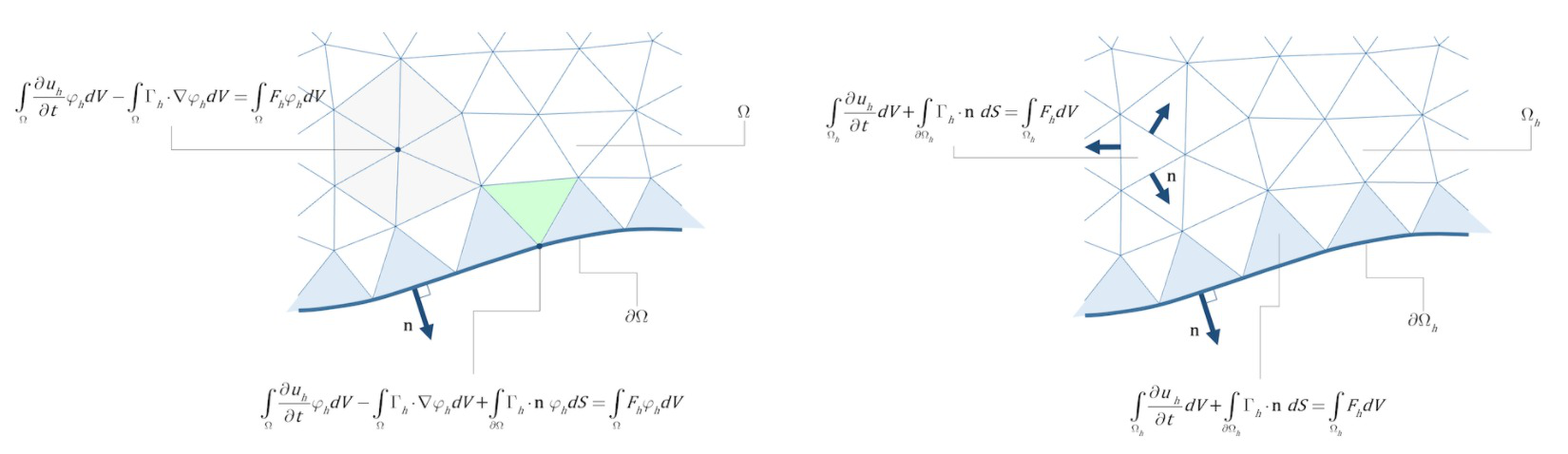
Fig. 2.1.2 Tsunami map across the world and color coded to the destructiveness of the earthquake and tsunami (Source: NOAA, Natural Hazards Viewer)

2.2. Discretization

The discretization procedure used in the FVM involves two steps, namely

• The integration of the PDE’s and their transformation into a form of the balance equations over a single element. This process involves modification of the integrals, both surface and volume, into discrete algebraic relations over elements.

• In the second step, interpolation profiles are chosen to approximate the value of variables inside the element. Further on, these interpolation profiles are used to related the cell values to the surface values.

In tihs technical manual, we will give a brief overview of both the procedures. A more detailed technical outlook can be found in the literature, [MoMaDa2016] .

General overview

FVM revolves around conservation of quantities such as mass, momentum and energy, typically associated with fluid mechanics problems. Since this method is based on applying conservation principles over each control volume, global conservation of each quantity is already ensured. One of the first objectives of FVM is discretization or dividing the physical domain into a finite number of small control volumes or cells. There is no restriction on the shape of the control volume although it is necessary that the resulting volume is convex and the faces that make up the control volume should be planar (3D) and bounded by straight edges (2D). All data about the control variables are stored at the centroid of each control volume and extra boundary nodes are often added for convenience.

2.3. Numerical integration

The conservation equation for any given general scalar variable \(\phi\) can be given as

(2.3.1)\[\underbrace{\frac{\partial \left( \rho \phi \right)}{\partial t}}_{\text{Transient term}} + \underbrace{\nabla \cdot \left( \rho \mathbf{v} \phi \right)}_{\text{Convective term}} = \underbrace{\nabla \cdot \left( \Gamma^{\phi} \nabla\phi \right)}_{\text{Diffusion term}} + \underbrace{Q^{\phi}}_{\text{Source term}}\]

where \(\rho\) is the density of the fluid, \(\mathbf{v}\) is the velocity vector. Considering the quasi-static flow, by dropping the transient term, and integrating over the volume of an element, we have

(2.3.2)\[\int_{\Omega} {\nabla \cdot \left(\rho\mathbf{v}\phi\right) \ d\Omega} = \int_{\Omega} {\nabla \cdot \left( \Gamma^{\phi} \nabla\phi \right) \ d\Omega} + \int_{\Omega} {Q^{\phi} \ d\Omega}\]

Using the divergence theorem, the above can be re-written in terms of surface integrals as

(2.3.3)\[\int_{\Gamma} {\left(\rho\mathbf{v}\phi\right) \ d\Gamma} = \int_{\Gamma} {\left( \Gamma^{\phi} \nabla\phi \right) \ d\Gamma} + \int_{\Omega} {Q^{\phi} \ d\Omega}\]

The above integral form requires the evaluation of the flux integration over the elemental faces for the convective and diffusion terms. This can be alternatively written as the summation of the flux terms over each of the individual faces of the element, i.e.

(2.3.4)\[\begin{split}\begin{split} \int_{\Gamma} {\left(\rho\mathbf{v}\phi\right) \ d\Gamma} &= \sum_{i = 1}^{n\left(\Omega\right)} \left( \int_{\Gamma_i} {\left(\rho\mathbf{v}\phi\right) \ d\Gamma} \right) \\ \int_{\Gamma} {\left( \Gamma^{\phi} \nabla\phi \right) \ d\Gamma} &= \sum_{i = 1}^{n\left(\Omega\right)} \left( \int_{\Gamma_i} {\left( \Gamma^{\phi} \nabla\phi \right) \ d\Gamma} \right) \end{split}\end{split}\]

where \(n\left(\Omega\right)\) represents the number of faces of the element with volume \(\Omega\), \(\Gamma_i\) represents the \(i\)-th face of the element with volume \(\Omega\). The above form of discretization ensures the conservation of quantities. It is important to note that the quantities of interest are conservative in nature. These include mass, volume, energy etc. Thus, without the convervative properties, the overall solution process can lead to unphysical solutions. In other words, the flux across the face of two shared elements need to have equal magnitudes but of opposite signs. The flux leaving the face of the first element should be equal to the flux entering, through the face, into the second element.

The resulting integral equations, shown above, include surface integral over each face of the element. These integral equations need to be converted to algebraic equations and are hence further simplified using the Gaussian quadrature as

(2.3.5)\[\int_{\Gamma_i} {\left( \alpha \right) \ d\Gamma} = \sum_{p} {\alpha_p w_p} A_{\Gamma_i}\]

where \(\alpha\) represents the quantity of interest (here the advection or diffusion term), \(A_{\Gamma_i}\) represents the area of the face, \(\alpha_p\) represents the quantity of interest at the \(p-th\) integration point, \(w_p\) represents the weight at the \(p-th\) integration point. The accuracy of the integration depends on the number of integration points used. In the case of a 2-D problem, the faces are 1-D line units and the integration points are given as

• One-integration point (or also known as Trapezoidal rule): \(\xi_{p} = 1\) and \(w_{p} = 1\)

• Two-integration points: \(\xi_{1} = \left(3-\sqrt{3}\right)/6, \ \xi_{2} = \left(3+\sqrt{3}\right)/6\) and \(w_{1} = w_{2} = 1/2\).

• Three-integration points: \(\xi_{1} = \left(5-\sqrt{15}\right)/10, \ \xi_{2} = 1/2, \ \xi_{3} = \left(5+\sqrt{15}\right)/10\) and \(w_{1} = 5/18, \ w_{2} = 4/9, \ w_{3} = 5/18\).

Similarly, the volume integration of the source term can be achieved using the Gaussian quadrature. Similar to the integration over the boundary, a volume integral need to be performed.

Once the PDE’s have been converted to a summation form above, it is necessary to express the face and volume fluxes in terms of the values of the variable at the neighboring cell centers or in otherwods, we need to linearize the fluxes.

2.4. Volume of fluid method

Volume of Fluid (VOF) was orignially presented by [HiNi1981] and is used extensively in modeling of multiphase flows. In our simulation of tsunami / storm-surge, we are working with water and air. However, VOF method is not restricted to two fluids but can also be used in the case of multiple fluids.

The VOF method is a numerical technique commonly used to track the free surface formed by the fluid-to-fluid interface. While, by itself, it is not a standalone flow solver, it only tracks and shape and evolution of the surface. It is solved in conjunction with the motion of the flow, described in the earlier sections.

Philosophy of VOF method

VOF uses the concept of volume fraction to weakly couple the transport equation with the continuity and momentum equations.

For every cell in the CFD domain, a volume fraction between zero to one is assigned. For example, in our case of tsunami/storm surge modeling, the volume fraction of one represents water, while zero represents air. Or in otherwords, if a cell is filled with only water, the volume fraction in that cell is one. In contrast, if it is only filled with air, the volume fraction in that cell is zero. For any cell that might have a combination of both water and air, the volume fraction rests between zero to one. To summarize, the volume fraction represents how much of the cell is occupied by each phase. In the case of multiple fluids, there are multiple volume fractions that need to be tracked.

The volume fraction is a variable that enters through the transport equations and need to be specified as boundary and initial conditions. Thus, if we have multiple volume fractions, there are multiples of these that need to be considered as well.

Mathematical formulation

A detailed treatise on the topic of VOF method, in particular with OpenFOAM, can be found in [Beetal2009] . Here, we will give a brief description of the ensuing mathematical formulations.

In the conventional VOF method, we consider

Continuity equation:

(2.4.1)\[\nabla \cdot \mathbf{v} = 0\]

Momentum equation:

(2.4.2)\[\frac{\partial \left(\rho \mathbf{v} \right)}{\partial t} + \nabla \cdot \left(\rho \mathbf{v} \mathbf{v} \right) = -\nabla p + \nabla \cdot \mathbf{T} + \rho \mathbf{f}_{b}\]

Transport equation:

(2.4.3)\[\frac{\partial \gamma}{\partial t} + \nabla \cdot \left( \mathbf{v} \gamma \right) = 0\]

where \(0 \le \gamma \le 1\) is the phase fraction, \(\mathbf{T}\) is the deviatoric stress tensor and given as \(\mathbf{T} = 2\mu\varepsilon - \frac{2\mu}{3} \left( \nabla \cdot \mathbf{v} \right)\), and the strain is \(\varepsilon = \frac{1}{2} \left( \nabla \cdot \mathbf{v} + \left( \nabla \cdot \mathbf{v} \right)^{T} \right)\), \(\mathbf{f}_{b}\) is the body forces per unit mass.

When the two fluids are considered immiscible, then they are considered as on effective fluid. The properties are calculated as the weighted average based on the distribution of the volume fractions. The properties are calculated as

• Density: \(\rho = \rho_{\ell} \gamma + \rho_{g} \left(1-\gamma\right)\)

• Viscosity: \(\mu = \mu_{\ell} \gamma + \mu_{g} \left(1-\gamma\right)\)

where \((\cdot)_{\ell}\) and \((\cdot)_{g}\) are the properties of the liquid and gas phase, respectively. However, in the case of flows with high-density ratios, it is possible that the conservation of phase fraction is not conserved. Violation of the phase conservation can lead to inaccurate phase distribution, surface curvature and thus corresponding pressure gradients across the free surface. However, unfortunately, it is not straight-forward to assure the conservativeness of the phase. It is not easy to determine the contributions of the velocity of each phase on the interface. Thus, the interface layer is smeared over a few grid cells and sensitive to grid resolution.

Thus, improper calculation of the surface curvature.

Points to note

• One other aspect that needs to be considered is the effect of hydrostatic pressure. Thus, one also needs to consider which direction the gravity is pointed in.

2.5. References

MoMaDa2016

6. Moukalled, L. Mangani and M. Darwish, “The finite volume method in computational fluid dynamics,” Springer International Publishing Switzerland (2016)

HiNi1981

3. 23. Hirt and B. D. Nichols , “Volume of fluid (VOF) method for the dynamics of free boundaries,” Journal of Computational Physics, vol. 39(1), pp. 201-225 (1981)

Beetal2009

5. Berberovic, N. P. Van Hinsberg, S. Jakirlic, I. V. Roisman, C. Tropea, “Drop impact onto a liquid layer of finite thickness: Dynamics of the cavity evolution,” Physical Review E, vol. 79 (2009)