4.2. Shear Building: HAZUS Assessment
This study explores a simple uncertainty propagation problem in the following three story shear building and employs the HAZUS methodology for assessing damage and loss:
Fig. 4.2.1 Three Story Shear Building Model (P10.2.9, “Dynamics of Structures”, A.K.Chopra)
This example uses the PBE application to automatically prepare an column model that represents the three-story structure, subject it to a suite of ground motion time histories, and evaluate the seismic performance of the building using the Hazus Earthquake methodology.
Each step of the workflow for this problem is explained below by sequentially walking through the input panels and highlighting their role in the simulation. The file input.json contains all of the settings for this exercise. It can be opened (using File/Open) to automatically populate the fields in the user interface.
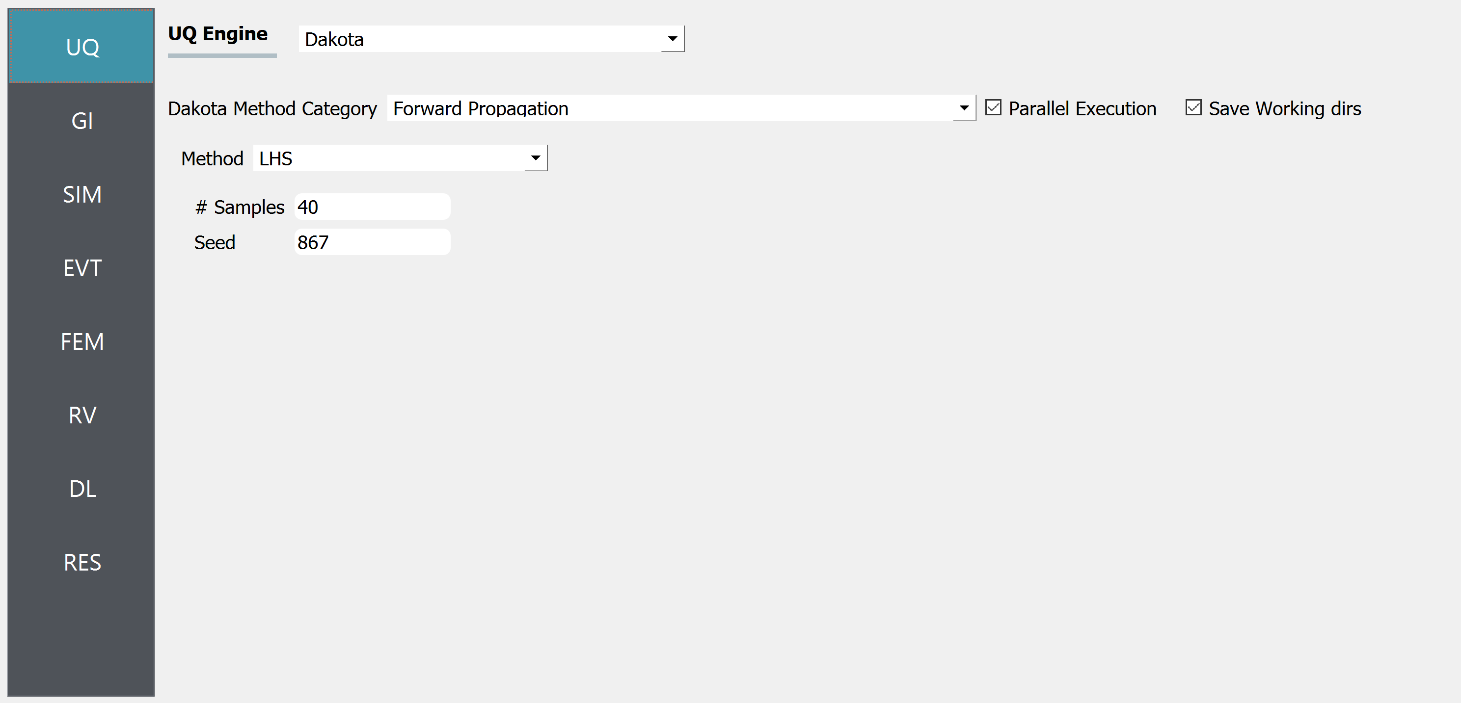
4.2.1. Step 1: UQ
This panel provides an interface to various forward propagation procedures which are used to sample the random variables defined in later panels and propagate each realization through the workflow. This process can be used to characterize the uncertainty in the workflow outputs. For this example, a latin hypercube sampling procedure (LHS) is used with 40 samples and a seed of 775. Fixing the seed ensures the same random sample every time the calculation is run.
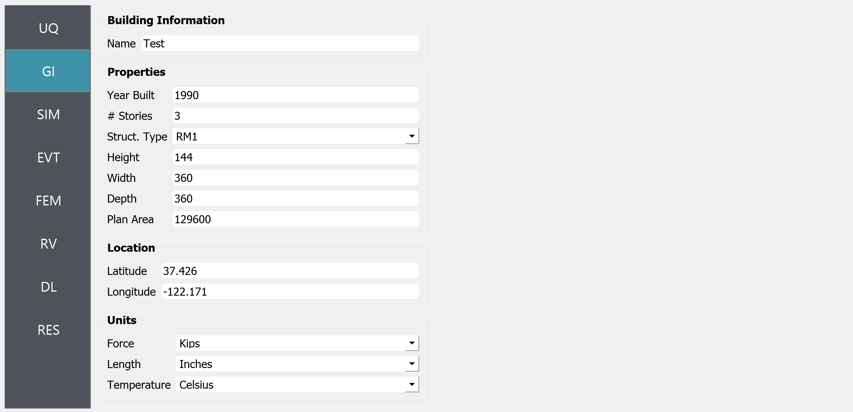
4.2.2. Step 2: GI
Next, the GI panel may be used to define metadata and other general information about the model. Some of the values are automatically updated by later panels while others are only providing information about the model and not used for the simulation.
It is important to review and specify the desired Units for the calculation here. It is important to provide all inputs assuming these units when no other instructions are given by the following panels. The length unit is used to define velocity and acceleration units as well.
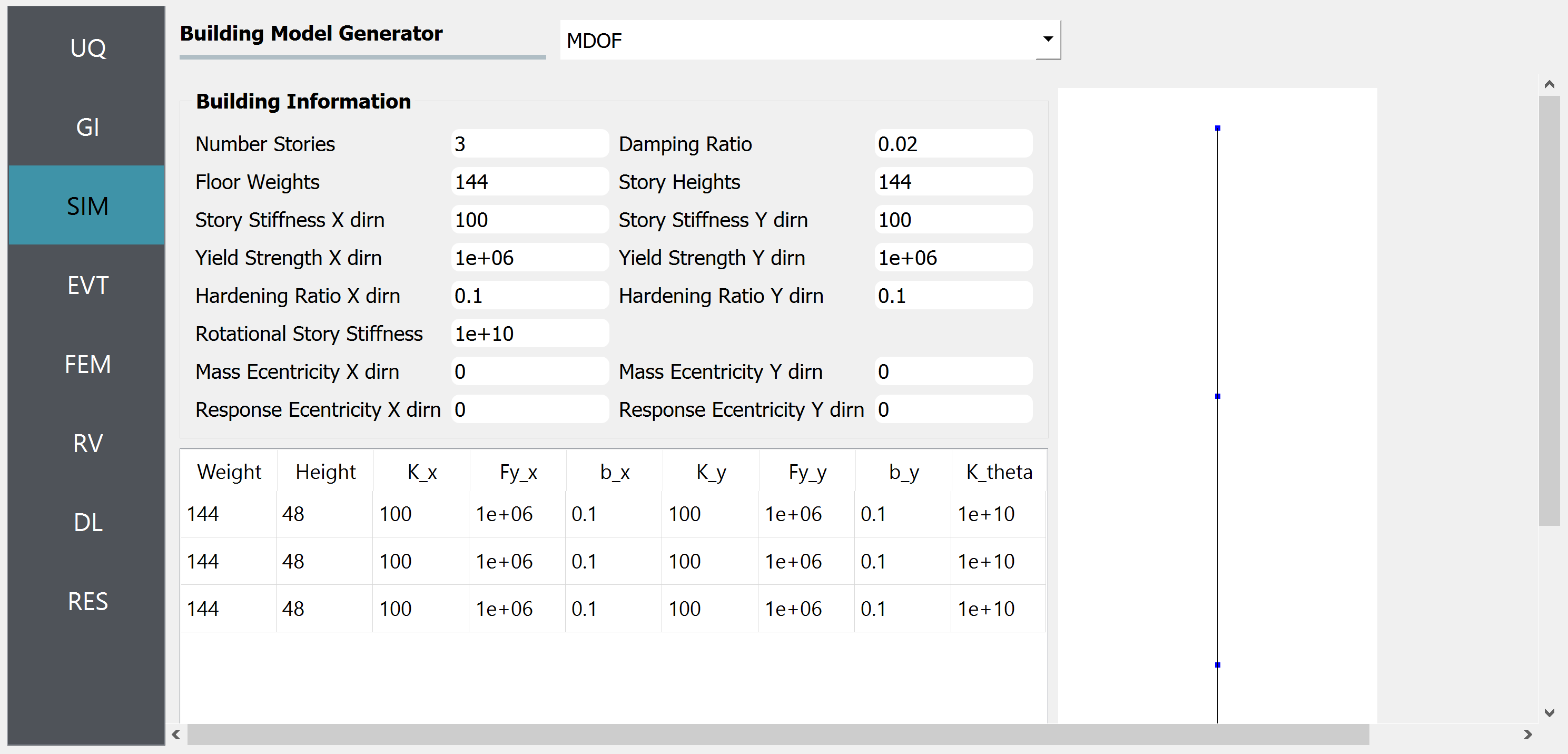
4.2.3. Step 3: SIM
The SIM panel can be used to define the simulation model. In this example we leverage the convenient MDOF tool which provides a high-level interface for defining simple parameterized structural analysis models. Either variable names, or literal values can be entered in the fields of this panel, as shown in the following figure.
This model could have random properties that we could sample and propagate the corresponding uncertainty through the workflow. If a variable name is entered, PBE automatically identifies it as a random variable, and creates a corresponding entry in the RV panel. Several examples in the documentation of the EE-UQ application demonstrate this feature on models of various complexity. In this example, we use a deterministic structural model for the sake of simplicity.
4.2.4. Step 4: EVT
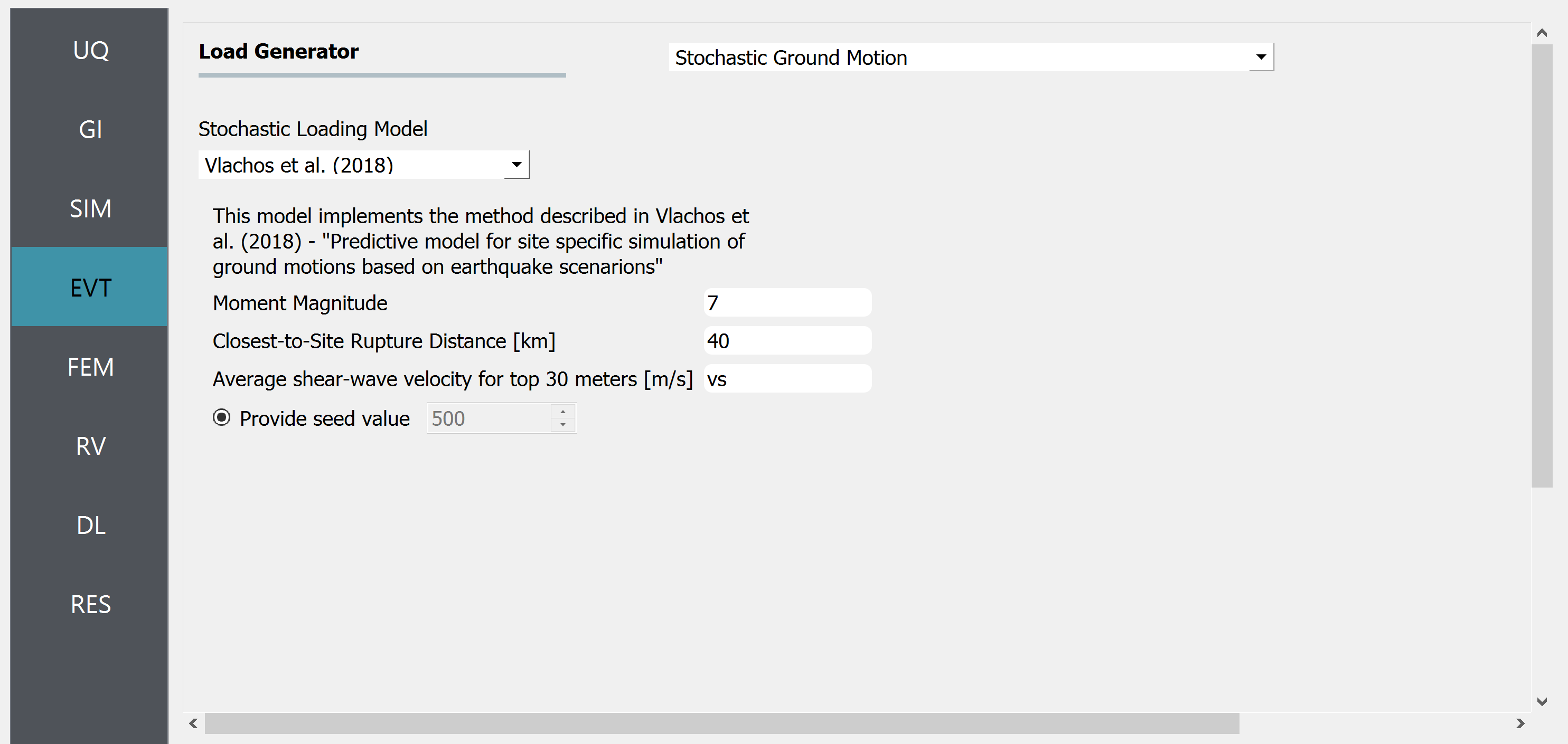
The EVT panel provides various Load Generator options that can either import ground motion loads from external files or connect to the PEER NGA database and obtain loads that represent a target spectrum or generate loads during the simulation using a stochastic process. We will use the latter solution in this example by selecting the Stochastic Ground Motion option.
The Vlachos et al. (2018) model generates ground motion time histories based on three parameters: magnitude, distance, and shear-wave velocity in the top 30 meters of the soil. We specify a magnitude 7 earthquake 40 kms from the site of interest. As for the shear-wave velocity, we introduce a random variable by providing vs as input. This is recognized by PBE and the corresponding variable is automatically added to the RV panel.
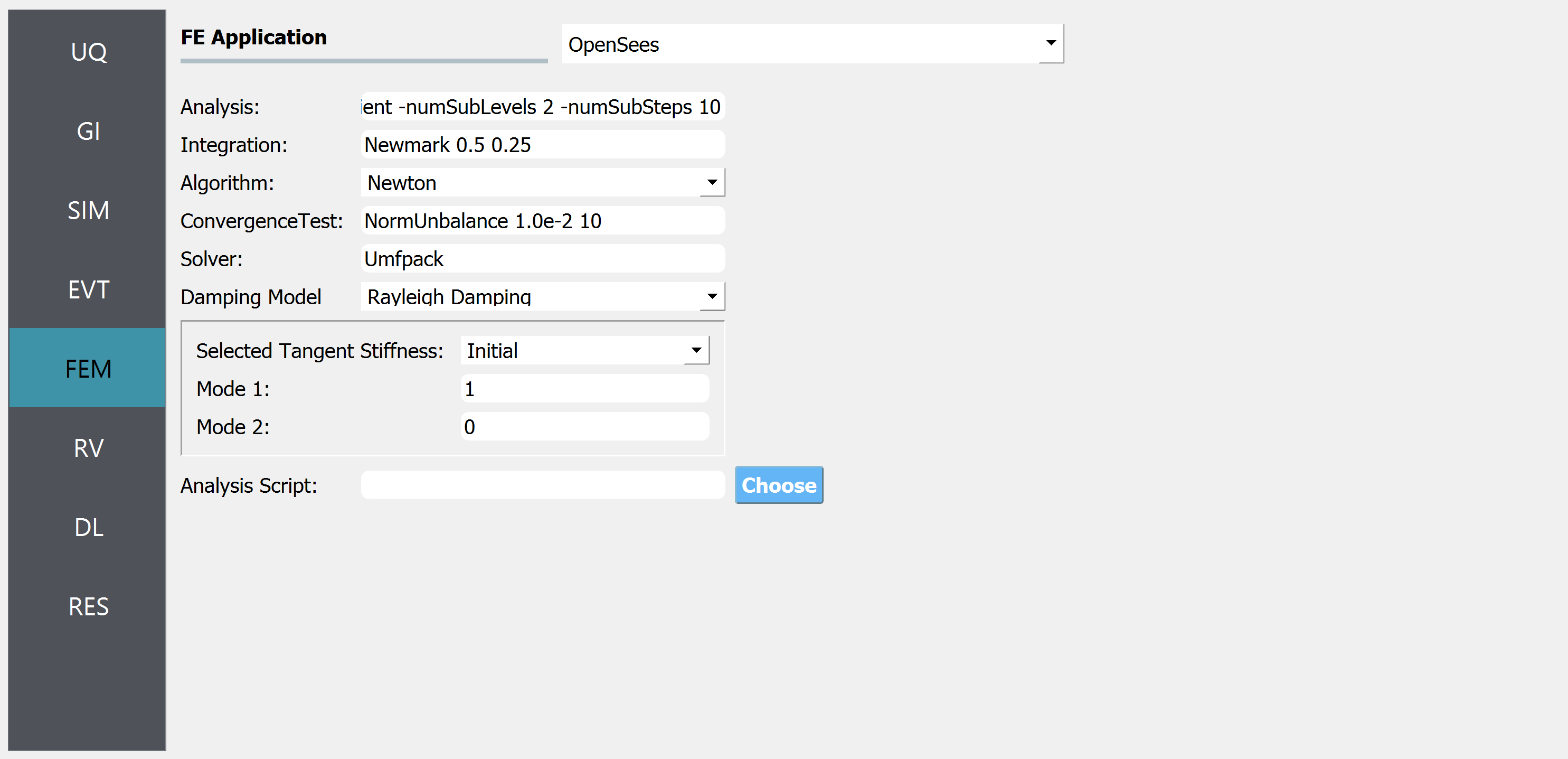
4.2.5. Step 5: FEM
We now proceed to the FEM panel where we can adjust settings for running the dynamic analysis. The default settings are typically appropriate for analyses that use the MDOF tool.
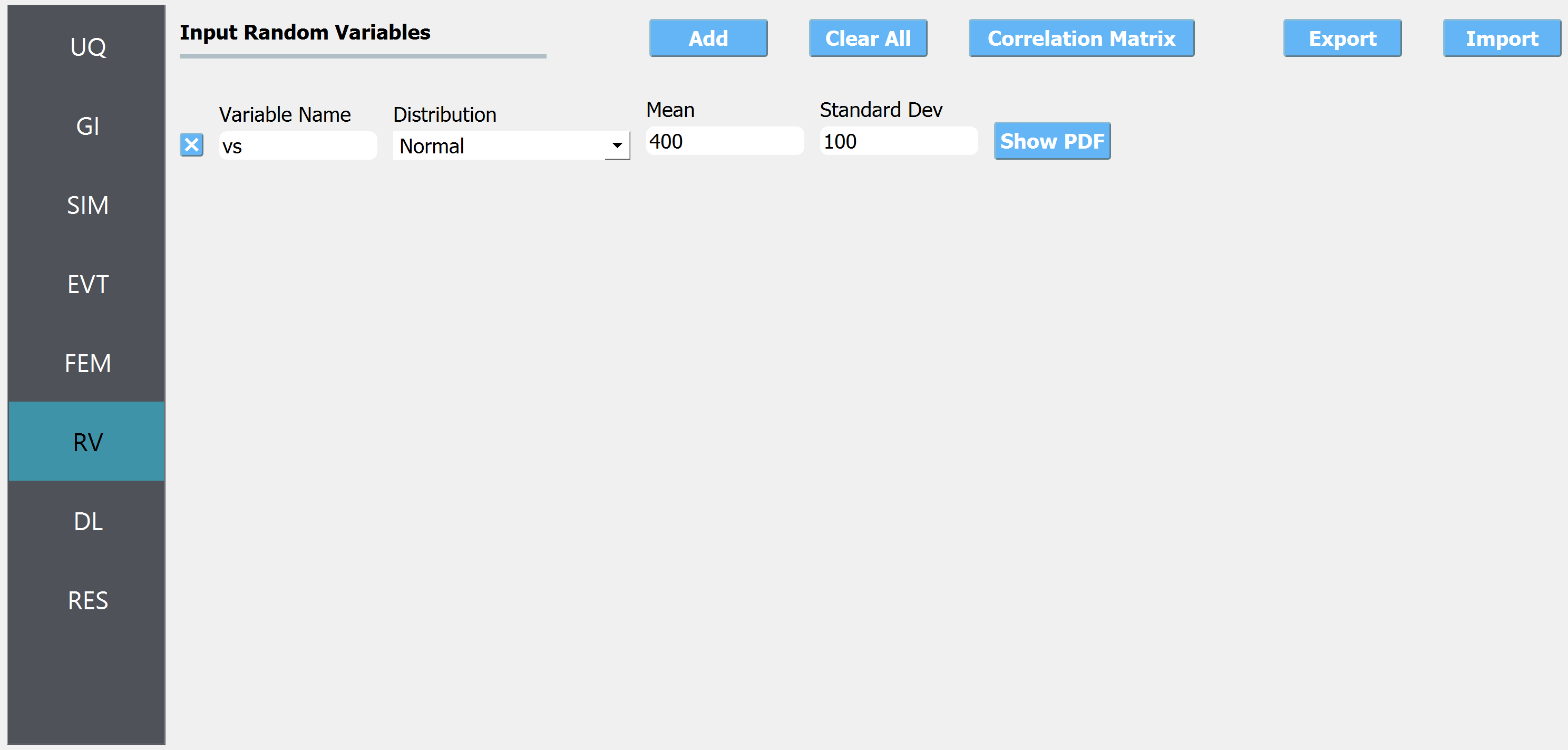
4.2.6. Step 6: RV
Now in the RV panel we will enter the distributions and values for our random variables. Because of the steps we have followed and entries we have made, when this tab is opened it already contains the vs random variable. We choose to model the uncertainty in the shear wave velocity using a normal distribution with a mean of 400 m/s and a standard deviation of 100 m/s.
Warning
Do not leave any of the distributions for these values as constant when using the Dakota UQ engine.
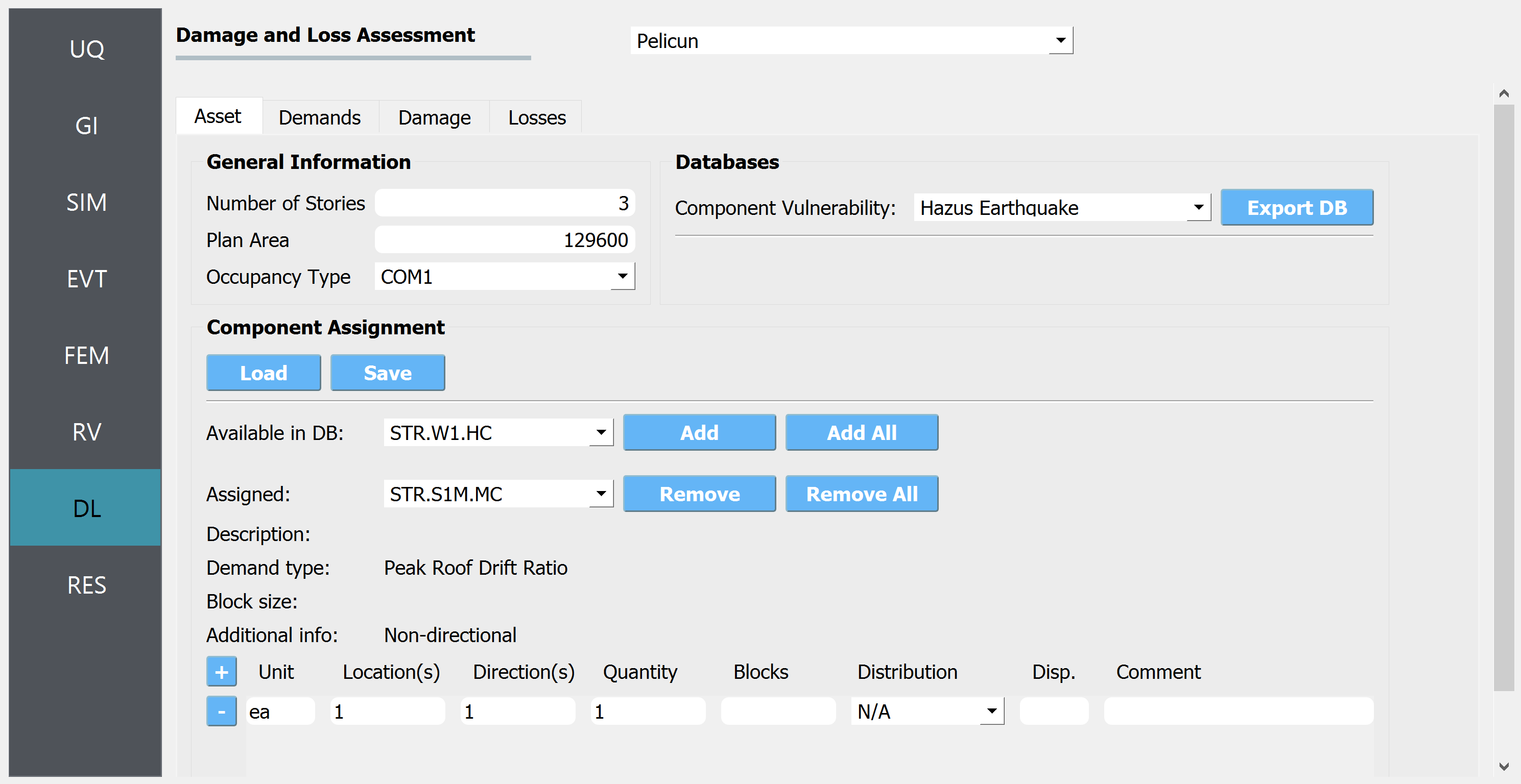
4.2.7. Step 7: DL
The last step in the setup is the DL panel. We use the four tabs in this panel to specify the performance model following the Hazus Earthquake methodology.
First, in the Asset tab, we choose the Hazus Earthquake component vulnerability database that is bundled with the PBE application. This loads all of the building archetypes handled by Hazus in the Available in DB list. We assign the STR.S1M.MC steel frame archetype as the structural component. NSD and NSA.MC components are added to represent drift and acceleration-sensitive non-structural components.
Because Hazus components are assigned at the building level, there is only one performance group created for each. The acceleration-sensitive component is assigned to the roof of the building (to obtain roof acceleration from there) while the drift-sensitive components are assigned to the first floor. This latter assignment is used with roof drift EDPs in buildings regardless of the number of floors they have.
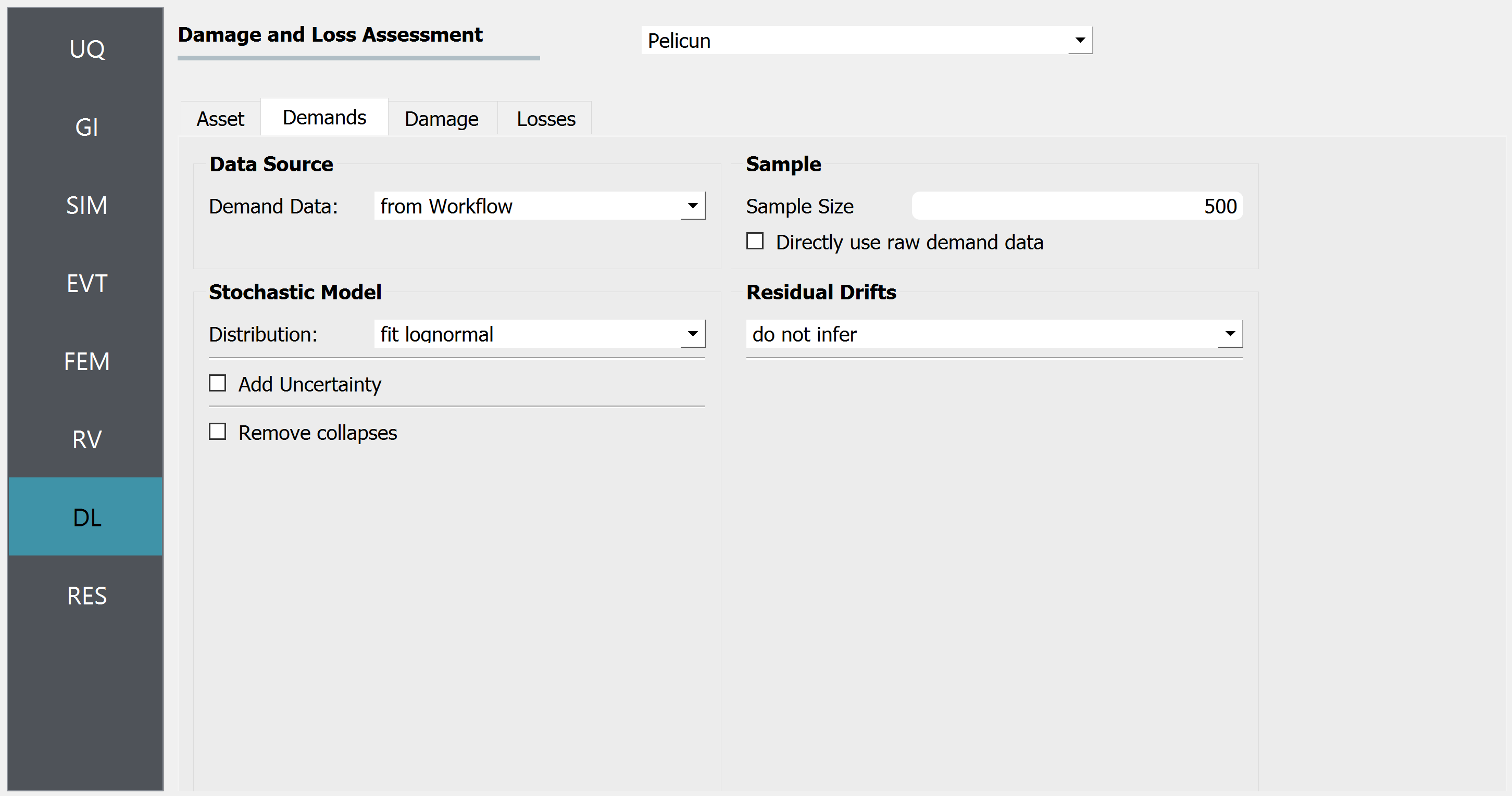
Under the Demands tab, we specify that the demand data is provided by the Workflow automatically; we assume that demands follow a multivariate lognormal distribution. After fitting such a distribution to the data, we sample 500 demand realizations for damage and loss assessment.
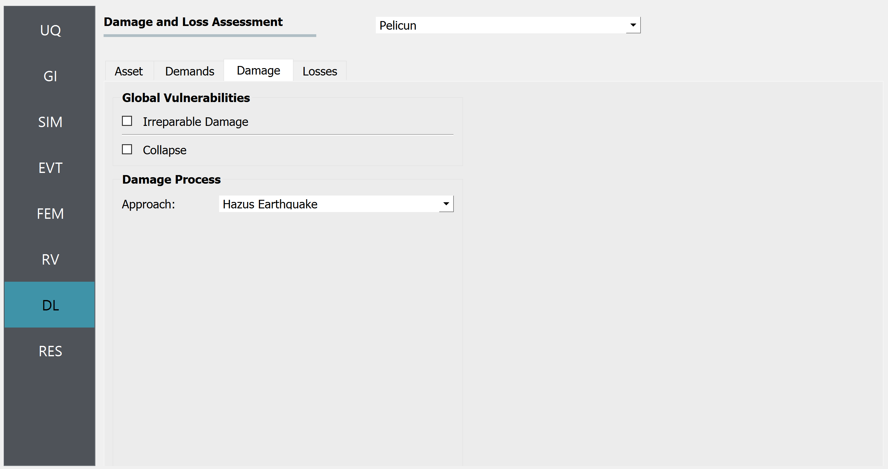
The Damage tab setup is simple when the Hazus earthquake methodology is used because this method includes collapse in the structure component damage states and does not consider irreparable damage. The Damage Process employed by this method is included in PBE and selected for this example.
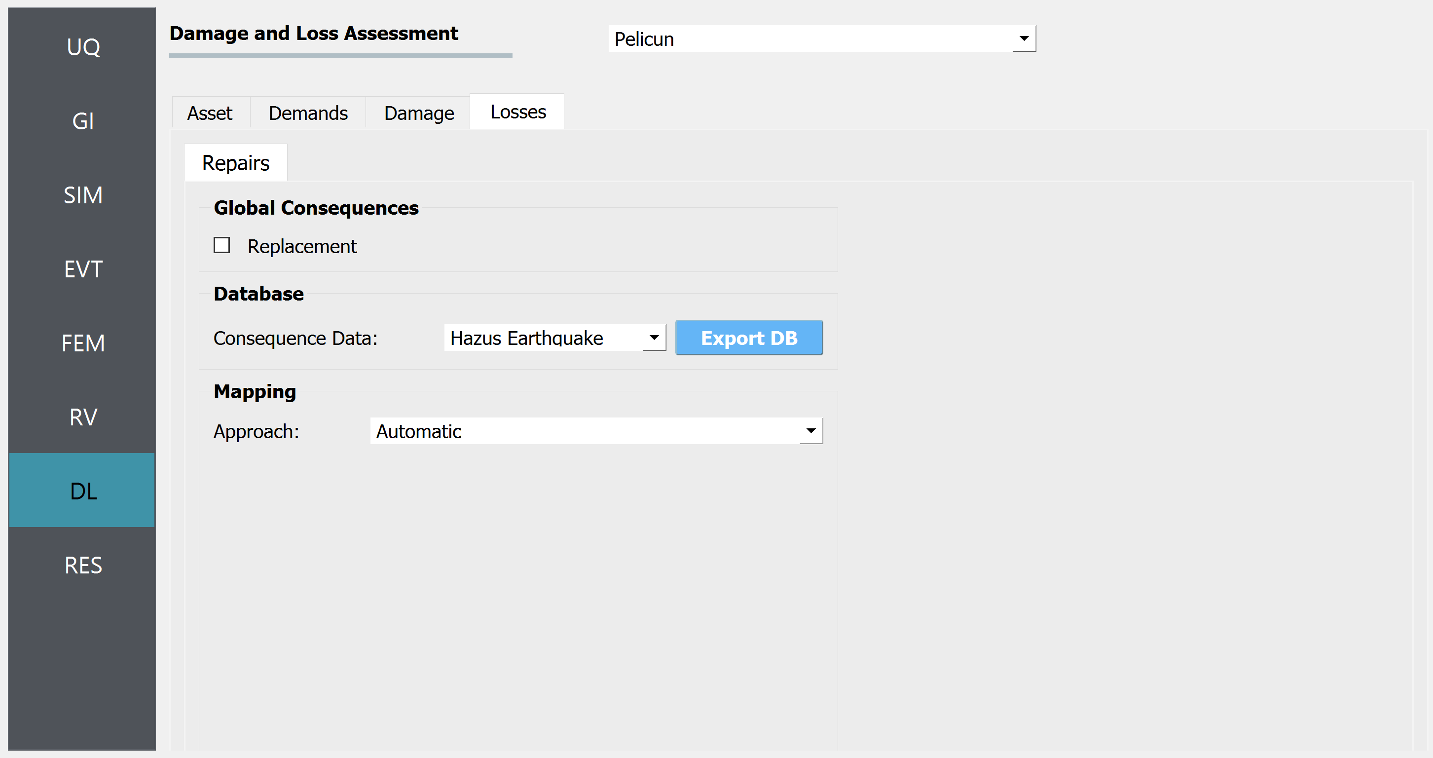
Losses are calculated using the included Hazus Earthquake consequence functions for repair costs and an Automatic mapping between damaged components and consequence models. This mapping uses the occupancy type and component types specified in the Asset tab earlier and selects the corresponding consequence functions following the Hazus methodology.
4.2.8. Analysis & Results
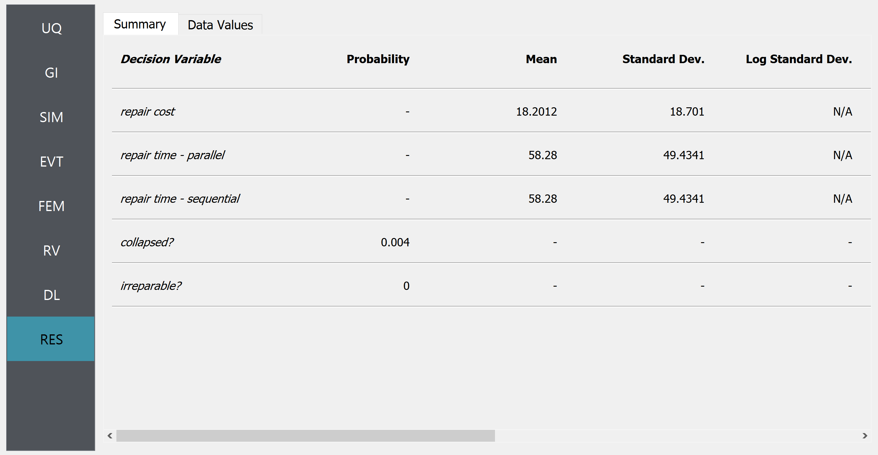
Once a full workflow has been defined click on the Run button. When the analysis is complete the RES tab will be activated and the results will be displayed. When a HAZUS assessment has been conducted, the results panel will resemble the following figures which show the Summary and Data tabs, respectively.
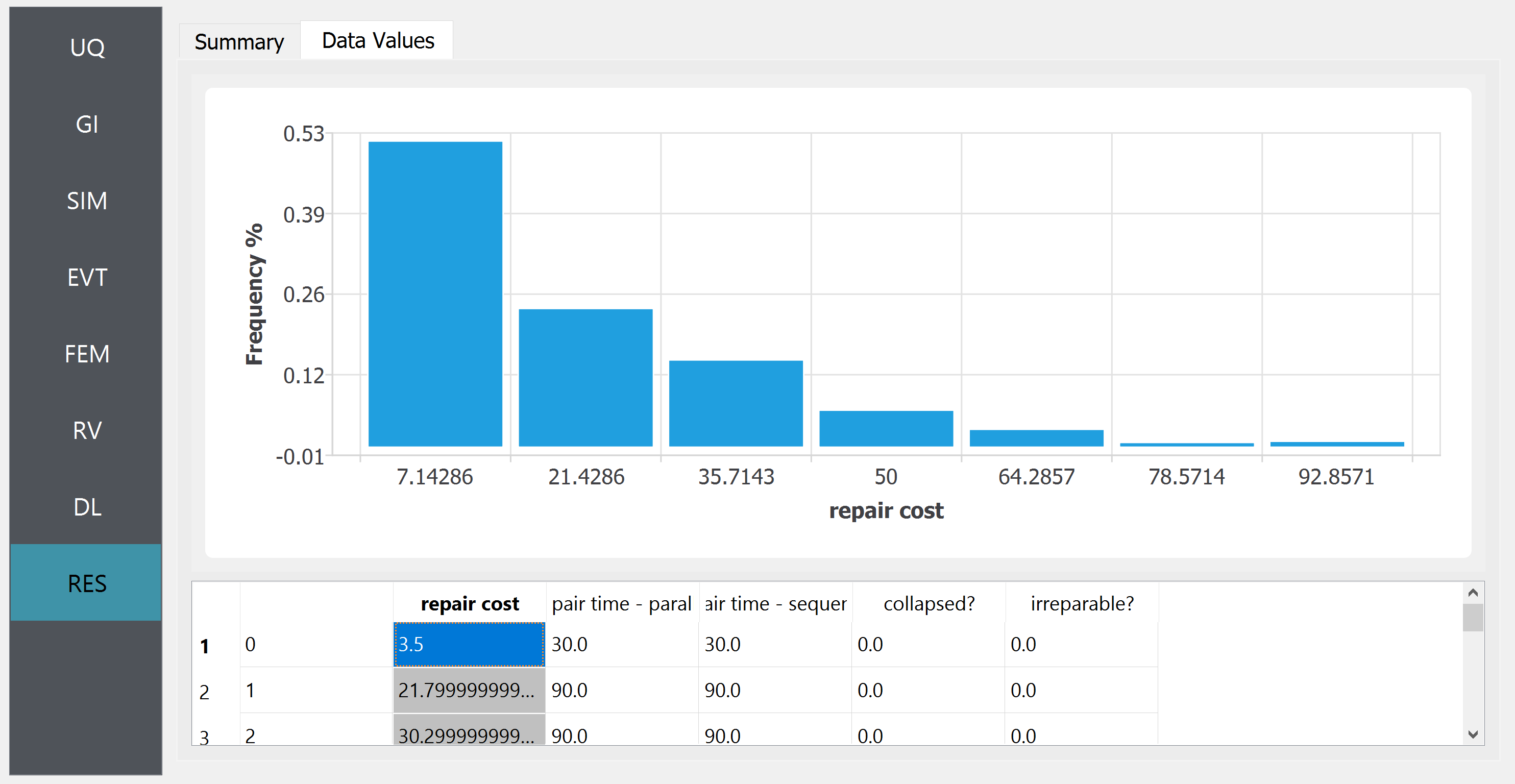
In the Data tab of the RES panel, we are presented with both a graphical plot and a tabular listing of the data. By left- and right-clicking on the individual columns the plot axis changes (left mouse click controls vertical axis, right mouse click the horizontal axis). If a singular column of the tabular data is selected with both right and left mouse buttons, a frequency and CDF plot will be displayed.