2.6. MOD: Asset Modeling
This section outlines how users can configure the modeling of various asset classes within the application. Users can choose specific applications for modeling different asset types, such as Buildings or Transportation Networks, via the Asset Selection Ribbon on the left-hand side of the interface, as depicted in Fig. 2.6.1. This ribbon is initially hidden and becomes visible when multiple asset types are selected in the GI: General Information panel. Only assets marked in the GI: General Information panel will be displayed in the Asset Selection Ribbon. Switching between assets updates the Input Panel to show the relevant applications for modeling the selected asset type.
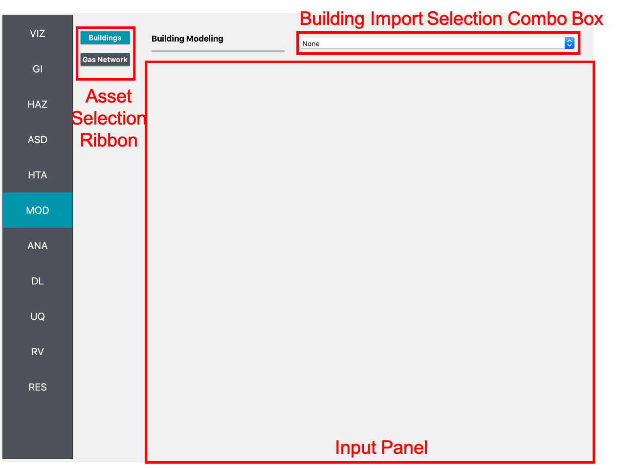
Fig. 2.6.1 Buildings modeling input panel.
2.6.1. Buildings
For building modeling, the following applications are available:
MDOF-LU Building Model
OpenSeesPy Building Model
2.6.1.1. MDOF-LU Building Model
The MDOF-LU application generates a hysteretic, multi-degree of freedom (MDOF) model based on high-level building information provided by the user. This approach is adapted from [Lu2020]. It processes building inventory data (e.g., construction year, structural type, plan area, number of stories) provided by the user in the ASD tab to determine the design code level and generates an OpenSees model for each building. Required information includes:

Hazus Data File: Path to a file with rules mapping design code levels and structural types to structural parameters. An example file can be downloaded
here, with column names explained below:Column names of HazusData.txt (click)
Table 2.6.1.1.1 Column names of HazusData.txt (showing the first 10 rows for high-code)¶ id
str type
min #story
max #story
height
Sy
eta
C
gamma
eta_soft
alpha
beta
a_k
omega
damage1
dmamge2
damage3
damage4
T1
T2
hos
damp
1
W1
1
50
18.4547
0.4
0.0870354
1000
0.8
-0.001
3
1
0.1
0.2
0.004
0.012
0.04
0.1
0.35
0.33333
4.27
0.1
2
W2
1
50
56.243
0.4
0.0794118
1000
0.6
-0.001
2.5
1
0.1
0.2
0.004
0.012
0.04
0.1
0.2
0.33333
3.66
0.1
3
S1L
1
3
38.7247
0.25
0.0865974
1000
1
-0.001
3
1
0
0.2
0.006
0.012
0.03
0.08
0.25
0.33333
3.66
0.05
4
S1M
4
7
51.7562
0.156
0.133734
1000
1
-0.001
3
1
0
0.2
0.004
0.008
0.02
0.0533
0.216
0.33333
3.66
0.05
5
S1H
8
50
62.9659
0.098
0.181032
1000
1
-0.001
3
1
0
0.2
0.003
0.006
0.015
0.04
0.17
0.33333
3.66
0.05
6
S2L
1
3
56.243
0.4
0.0670927
1000
0.5
-0.001
2
1
0
0.2
0.005
0.01
0.03
0.08
0.2
0.33333
3.66
0.05
7
S2M
4
7
75.8694
0.333
0.103936
1000
0.5
-0.001
2
1
0
0.2
0.0033
0.0067
0.02
0.0533
0.172
0.33333
3.66
0.05
8
S2H
8
50
85.0452
0.254
0.142936
1000
0.5
-0.001
2
1
0
0.2
0.0025
0.005
0.015
0.04
0.136154
0.33333
3.66
0.05
9
S3
1
50
14.0607
0.4
0.0670927
1000
1
-0.001
2
1
0
0.2
0.004
0.008
0.024
0.07
0.4
0.33333
4.57
0.05
10
S4L
1
3
74.5959
0.32
0.0727412
1000
0.5
-0.001
2.25
1
0
0.2
0.004
0.008
0.024
0.07
0.175
0.33333
3.66
0.05
See Fig. 2.6.1.1.1 for the parameter definitions. Note that not all the parameters are being used.
Std deviation Stiffness: Standard deviation for lateral stiffness. The uncertainty will be applied by sampling a multiplication factor with the specified standard deviation and mean of 1. The factor is sampled only once per structure and will be applied to all stories.
Std deviation Damping: Standard deviation for damping ratio. The uncertainty will be applied by sampling a multiplication factor with the specified standard deviation and mean of 1.
Default Story Height (optional): Sets mass node coordinates.
The analysis outputs include a SAM.json file for structural parameters and an example.tcl file (with uniaxialMaterial Hysteretic material model) for the downstream OpenSees model. Both files are located in the working directory.
Example of SAM.json (click)
{
    "Properties":
    {
        "dampingRatio": 0.09956333887469665,
        "uniaxialMaterials":
        [
            {
                "name": 1,
                "type": "shear",
                "K0": 61532397.052015901,
                "Sy": 2110124.6849974156,
                "eta": 0.087035399999999999,
                "C": 1000.0,
                "gamma": 0.80000000000000004,
                "alpha": 3.0,
                "beta": 1.0,
                "omega": 0.20000000000000001,
                "eta_soft": -0.001,
                "a_k": 0.10000000000000001
            },
            {
                "name": 2,
                "type": "shear",
                "K0": 61532397.052015901,
                "Sy": 1406749.7899982773,
                "eta": 0.087035399999999999,
                "C": 1000.0,
                "gamma": 0.80000000000000004,
                "alpha": 3.0,
                "beta": 1.0,
                "omega": 0.20000000000000001,
                "eta_soft": -0.001,
                "a_k": 0.10000000000000001
            }
        ]
    },
    "Geometry":
    {
        "nodes":
        [
            {
                "name": 1,
                "crd":
                [
                    0.0,
                    0.0,
                    0.0
                ],
                "ndf": 6,
                "constraints":
                [
                    1,
                    1,
                    1,
                    1,
                    1,
                    1
                ]
            },
            {
                "name": 2,
                "mass": 284190.39936000004,
                "crd":
                [
                    0.0,
                    0.0,
                    3.6000000000000001
                ],
                "ndf": 6,
                "constraints":
                [
                    0,
                    0,
                    1,
                    1,
                    1,
                    1
                ]
            },
            {
                "name": 3,
                "mass": 284190.39936000004,
                "crd":
                [
                    0.0,
                    0.0,
                    7.2000000000000002
                ],
                "ndf": 6,
                "constraints":
                [
                    0,
                    0,
                    1,
                    1,
                    1,
                    1
                ]
            }
        ],
        "elements":
        [
            {
                "name": 1,
                "type": "shear_beam2d",
                "uniaxial_material": 1,
                "nodes":
                [
                    1,
                    2
                ]
            },
            {
                "name": 2,
                "type": "shear_beam2d",
                "uniaxial_material": 2,
                "nodes":
                [
                    2,
                    3
                ]
            }
        ]
    },
    "NodeMapping":
    [
        {
            "cline": "response",
            "floor": "0",
            "node": 1
        },
        {
            "cline": "response",
            "floor": "1",
            "node": 2
        },
        {
            "cline": "response",
            "floor": "2",
            "node": 3
        }
    ],
    "units":
    {
        "force": "kN",
        "length": "m",
        "temperature": "C",
        "time": "sec"
    }
}
Example of opensees.tcl (click)
model BasicBuilder -ndm 3 -ndf 6
node 1 0 0 0
fix 1 1 1 1 1 1 1
node 2 0 0 3.6 -mass 284190 284190  0.0  0.0  0.0 2.8419e-05
fix 2 0 0 1 1 1 1
node 3 0 0 7.2 -mass 284190 284190  0.0  0.0  0.0 2.8419e-05
fix 3 0 0 1 1 1 1
uniaxialMaterial Hysteretic 1 2.11012e+06 0.0342929 6.33037e+06 0.822315 6.33037e+06 1 -2.11012e+06 -0.0342929 -6.33037e+06 -0.822315 -6.33037e+06 -1 0.8 0.8 0 0 0.1
uniaxialMaterial Hysteretic 2 1.40675e+06 0.0228619 4.22025e+06 0.54821 4.22025e+06 1 -1.40675e+06 -0.0228619 -4.22025e+06 -0.54821 -4.22025e+06 -1 0.8 0.8 0 0 0.1
element zeroLength 1 1 2 -mat 1 1 -dir 1 2
element zeroLength 2 2 3 -mat 2 2 -dir 1 2
loadConst -time 0.0
#timeSeries Path 101 -dt 0.005 -factor [expr 1 * 1 * 1 ] -values { -1.46509e-05 8.24738e-06 -2.26001e-05 1.46955e-05 -2.63045e-05 ..... -3.42224e-05  }
#timeSeries Path 102 -dt 0.005 -factor [expr 1 * 1 * 1 ] -values { 7.15223e-06 -2.4271e-05 1.94678e-05 -3.62861e-05 2.96503e-05 ...... -0.000675427  }
pattern UniformExcitation 101 1 -fact 1 -accel 101
set numStep 60000
set dt 0.005
pattern UniformExcitation 102 2 -fact 1 -accel 102
set numStep 60000
set dt 0.005
set numberOfStories 2
recorder EnvelopeNode -file 1-AIM.json0.max_abs_acceleration.response.0.out -timeSeries 101 102  -node 1 -dof 1 2  accel
recorder EnvelopeNode -file 1-AIM.json0.max_abs_acceleration.response.1.out -timeSeries 101 102  -node 2 -dof 1 2  accel
recorder EnvelopeNode -file 1-AIM.json0.max_rel_disp.response.1.out -node 2 -dof 1 2  disp
recorder EnvelopeDrift -file 1-AIM.json0.max_drift.response.0.1.1.out -iNode 1 -jNode 2 -dof 1 -perpDirn 3
recorder EnvelopeDrift -file 1-AIM.json0.max_drift.response.0.1.2.out -iNode 1 -jNode 2 -dof 2 -perpDirn 3
recorder EnvelopeNode -file 1-AIM.json0.max_abs_acceleration.response.2.out -timeSeries 101 102  -node 3 -dof 1 2  accel
recorder EnvelopeNode -file 1-AIM.json0.max_rel_disp.response.2.out -node 3 -dof 1 2  disp
recorder EnvelopeDrift -file 1-AIM.json0.max_drift.response.1.2.1.out -iNode 2 -jNode 3 -dof 1 -perpDirn 3
recorder EnvelopeDrift -file 1-AIM.json0.max_drift.response.1.2.2.out -iNode 2 -jNode 3 -dof 2 -perpDirn 3
recorder EnvelopeDrift -file 1-AIM.json0.max_roof_drift.response.0.2.1.out -iNode 1 -jNode 3 -dof 1 -perpDirn 3
recorder EnvelopeDrift -file 1-AIM.json0.max_roof_drift.response.0.2.2.out -iNode 1 -jNode 3 -dof 2 -perpDirn 3

# Perform the analysis
numberer RCM
constraints Transformation
system Umfpack
integrator Newmark 0.5 0.25
test NormUnbalance 1.0e-2 10
algorithm Newton
analysis Transient -numSubLevels 2 -numSubSteps 10
set xDamp 0.0995633;
set lambdaN [eigen 3];
set lambdaI [lindex $lambdaN [expr 1 -1]];
set lambdaJ [lindex $lambdaN [expr 3 -1]];
set lambda1 [lindex $lambdaN 0]
set omega1 [expr pow($lambda1,0.5)];
set omegaI [expr pow($lambdaI,0.5)];
set omegaJ [expr pow($lambdaJ,0.5)];
set alphaM [expr $xDamp*(2*$omegaI*$omegaJ)/($omegaI+$omegaJ)];
set betaKinit [expr 0 *2.0*$xDamp/($omegaI+$omegaJ)];
set betaKcomm [expr 0 *2.0*$xDamp/($omegaI+$omegaJ)];
set betaKcurr [expr 1 *2.0*$xDamp/($omegaI+$omegaJ)];
rayleigh $alphaM $betaKcurr $betaKinit $betaKcomm;
set lambdaN [eigen 1];
set lambda1 [lindex $lambdaN 0]
set T1 [expr 2*3.14159/$lambda1]
set dTana [expr $T1/20.]
if {$dt < $dTana} {set dTana $dt}
analyze [expr int($numStep*$dt/$dTana)] $dTana
remove recorders
where the keys of SAM.json are defined as follows:

Fig. 2.6.1.1.1 Hysteresis model in MDOF-LU Building Model.
Note
When the MDOF-LU building modeling application is employed, the OpenSees simulation application should be used for analysis in the ANA: Asset Analysis input panel.
- Lu2020
Lu, X., McKenna, F., Cheng, Q., Xu, Z., Zeng, X., & Mahin, S. A. (2020). An open-source framework for regional earthquake loss estimation using city-scale nonlinear time history analysis. Earthquake Spectra, 36(2), 806-831.
2.6.1.2. OpenSeesPy Building Model
The OpenSeesPy application allows for the creation of structural models using a user-defined Python script. The input panel (Fig. 2.6.1.2.1) provides fields for:
OpenSeesPy Script: Script containing the code to create the building model.
Node Response Mapping: By default, the workflow assumes X=1, Y=2, Z=3 mapping between the x,y,z directions and degrees of freedom, with x and y being the horizontal directions. This input allows you to define an alternative mapping by providing three numbers separated by commas in a string, such as ‘1, 3, 2’ if you wish to have y as the vertical direction.
Analysis Spatial Dimensions: Number of dimensions in the OpenSeesPy analysis.
Degrees-of-Freedom at Node: Number of degrees-of-freedom at each node.
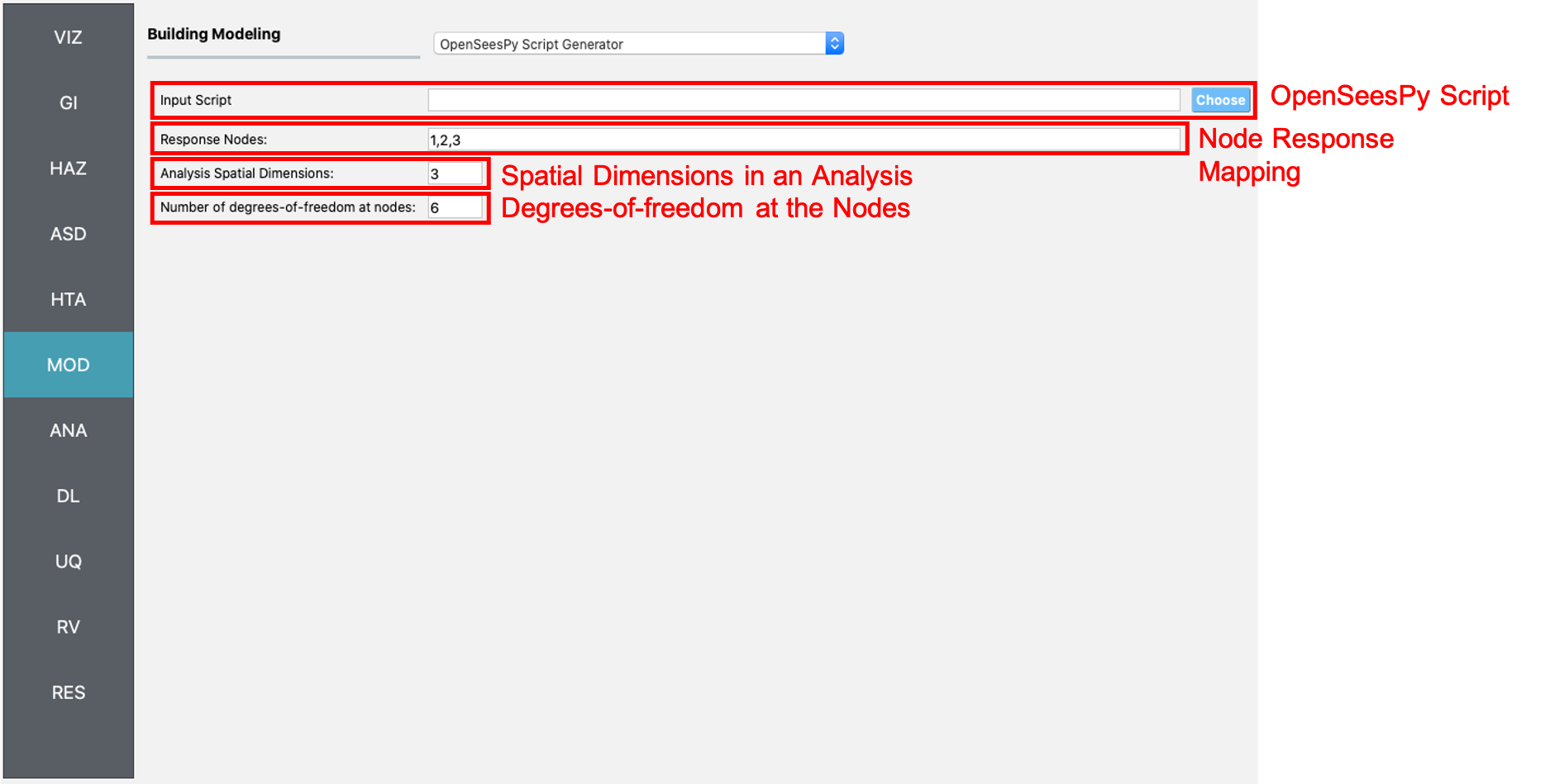
Fig. 2.6.1.2.1 OpenSeesPy Building model input panel.
2.6.2. Transportation Infrastructure
Currently, only Intensity Measure as Engineering Demand Parameter (IMasEDP) analysis is supported for transportation infrastructure. The asset models should be None for IMasEDP analyses.