Topography¶

There are three aspects to specifying the geometry in GeoClaw: (a) Bathymetry of the ocean floor and topography of the coastal area (b) Location and size of the fault of interest for tsunami simulation (c) Displacement of the fault.

Bathymetry¶

We will start by considering the specification of the bathymetric/topographic data. The bathymetry is assumed as a value of \(z\) (relative to a particular reference level) at each point \((x,y)\). Most often the water surface is considered as \(z=0\) for reference. In addition, GeoClaw recognizes only uniformly spaced rectangular bathymetry grids.

It should also be noted here that GeoClaw allows for multiple files to be input for the bathymetry. A bilinear interpolation is used to stitch the files to obtain the domain for the simulation. In regions of intersections, the best available information is used. This is further used to obtain a single top value related to the cell and used in the computations for solving the shallow water equations.

There are four formats supported by GeoClaw and SimCenter presently supports three of these formats as inputs to the Hydro-UQ tool. These formats are discussed below:

Topo type 01¶

The first format, known as topotype = 1 stores the \((x,y,z)\) points of all the points in the domain. The \((x,y)\) represent the latitude and longitude while the \(z\) represents the depth at the particular location. The size and spacing of the grid is thus obtained from the data directly. Each row, progressing from upper left corner (NW) and moving eastward. The next subsequent lines move southward. The files, generally, have the below format:

x1 y1 z1
x2 y2 z2
...
xn yn zn

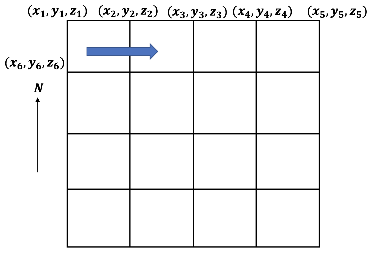
Fig. 3.1.1 Ordering of points as recorded in the files of type 01.¶

The points are ordered as illustrated in the above figure. The points start from the North-west part of the domain and progress east across the rows and later down.

Topo type 02¶

The second format, known as topotype = 2 is slightly more compact and stores only the \((z)\) value of all the points in the domain. It uses the fact that GeoClaw requires a regular and rectangular grid. The data related to the \((x,y)\) points (i.e. latitude and longitude) are derived from this header information given in the first six lines. The header information includes

value   mx
value   my
value   xlower / xllcenter / xllcorner
value   ylower / yllcenter / yllcorner
value   cellsize
value   nodataval
z1
z2
...

Here mx and my represent the number of points in the x- and y- directions; cellsize represent the size of the cell. All cells in the grid are of the same size and specified by either one value or by two values, i.e. dx and dy both. If there is a point \((x,y)\) on the grid, where the value of depth is not known, then the value specified using the value given as nodataval.

However, there are two aspects that can lead to ambiguity in reading the files, namely

The order of value and label can be in any order. Either it can be value followed by label or otherwise.
The third and fourth lines can either represent the value of the lower left corner, i.e. xlower and ylower or value of the lower left corner of the SW-most cell, i.e. xllcorner and yllcorner. Alternatively, it can also specify the center of this SW-most cell and represented by the labels xllcenter and yllcenter

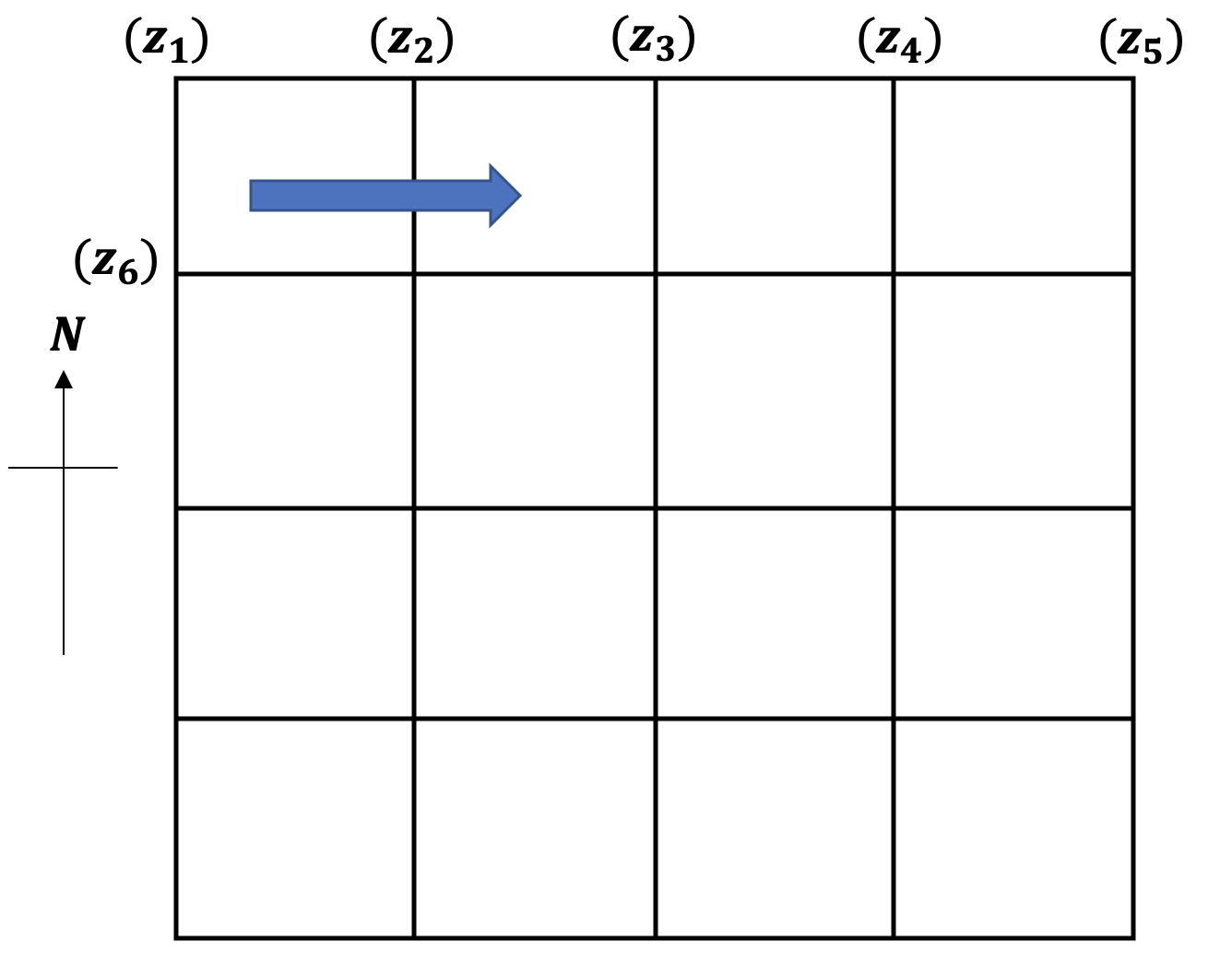
Fig. 3.1.2 Ordering of points as recorded in the files of type 02.¶

The points are ordered as illustrated in the above figure and is similar as that defined for the topo type 01 but here only the \((z)\) values are stored in the file. The points start from the North-west part of the domain and progress east across the rows and later down. The file has a total of mx*my number of lines in the file.

An example file will be as shown below

2      mx
2      my
0      xlower
-10    ylower
10     cellsize
9999   nodataval
-100
-200
-400
-250

Topo type 03¶

The third format, known as topotype = 3 is same as the ESRI ASCII Raster format .

The first six lines with the header for type 03 is same as for type 02. This is followed by my lines. Each of these lines contain mx values of \(z_i\) . This implies that the first line is the north-most line going from west to east and the last line is the south-most line going from west to east. The topo example file from type 2 can be written for type 03 and is given as below:

2      mx
2      my
0      xlower
-10    ylower
10     cellsize
9999   nodataval
-100 -200
-400 -250

Download topo files¶

Alternatively, there are several online databases that are available to download topography files for tsunami modeling. Some of these are given on the Clawpack website. This is achieved by downloading the file into the scratch folder using the maketopo.py file as

from clawpack.geoclaw import topotools
topo_fname = 'Name-of-topo.asc'
url = 'http://depts.washington.edu/clawpack/geoclaw/topo/etopo/' + topo_fname
clawpack.clawutil.data.get_remote_file(url, output_dir=scratch_dir,
        file_name=topo_fname, verbose=True)

Note¶

In types 2 and 3, the values and labels are interchangeable. However, the order of lines is important.
It is possible to automatically invert the z-values. This can be achieved by specifying the value of topotype as -1, -2 or -3.

Fault geometry¶

In order to simulate a scenario, an earthquake source needs to be specified. This is often given in terms of the slip of a fault plane or sub-faults that make up the single plane. This fault geometry is specified using parameters in the maketopo.py file as given below

usgs_subfault = dtopotools.SubFault()
usgs_subfault.strike = 16.
usgs_subfault.length = 450.e3
usgs_subfault.width = 100.e3
usgs_subfault.depth = 35.e3
usgs_subfault.slip = 15.
usgs_subfault.rake = 104.
usgs_subfault.dip = 14.
usgs_subfault.longitude = -72.668
usgs_subfault.latitude = -35.826
usgs_subfault.coordinate_specification = "top center"

Some of the important parameters for a single sub-fault are as shown in the figure below.

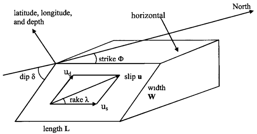
Fig. 3.1.3 Definition sketch of fault plane dimension and geometry (Source: E. Gica, M. H. Teng, P. L.-F. Liu and V. Titov, “Sensitivity analysis of source parameters for earthquake-generated distant tsunamis,” Journal of waterway, port, coastal and ocean engineering, vol. 133, pp. 429 - 441 (2007))¶

Each of the fault parameters are discussed, in detail, below.

Fault strike¶

The fault strike angle for a single sub-fault is specified using the command subfault_name.strike and is pitorially depicted in the below figure.

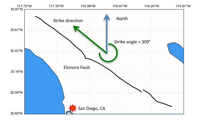
Fig. 3.1.4 Pictorial illustration of the strike angle (Source: http://schultz.physics.ucdavis.edu/research/fixing_faults.html)¶

In general, the strike line of a fault is a line representing the intersection of the feature with a horizontal plane. Here, this strike angle represents the slip direction of the fault and is measured clockwise from the north direction as shown in the above figure. This is generally between 0 - 360 degrees.

Fault dip¶

The dip of the sub-fault is specified using the command subfault_name.dip. This represents the steepest angle of descent of the fault relative to a horizontal plane, and is given by the number (\(0 - 90^o\)) as well as a letter (N,S,E,W) with rough direction in which the bed is dipping downwards.

One commonly used technique is to consider the strike so the dip is \(90^o\) to the right of the strike, in which case the redundant letter following the dip angle is omitted (right hand rule, or RHR). The map symbol is a short line attached and at right angles to the strike symbol pointing in the direction which the planar surface is dipping down. The angle of dip is included without the degree sign as, for example, subfault_name.dip = 14. This is specified is between 0 - 90 degrees positive.

Fault rake¶

The block below the fault plane is known as the Footwall while the one above is known as the Hangingwall. The rake angle represents the angle between the slip direction of the hangingwall block from the dip vector, as measured in the fault plane. This is specified, for example, as subfault_name.rake = 104. This is generally between - 180 to 180 degrees.

Fault dimensions and slip¶

The other dimensions of the sub-fault that needs to be specified include the length (subfault_name.length), width (subfault_name.width) and depth (subfault_name.depth) of the fault. This is often specified in meters or kilometers. Another important aspect is the slip of the fault given as subfault_name.slip and this represents the magnitube of slip along the rake. The slip is often specified in cm or m.

Fault location¶

The sub-fault location is specified in terms of latitude (subfault_name.latitude) and longitude (subfault_name.longitude) of a point on the fault plane. The location is also specified by the label subfault.coordinate_specification and the options include:

bottom center: (longitude,latitude) and depth specified at bottom center
top center: (longitude,latitude) and depth specified at top center
centroid: (longitude,latitude) and depth specified at the centroid of the fault plane
noaa sift: (longitude,latitude) specified at the bottom center while the depth is specified at top, This mixed convention is used by the NOAA SIFT database
top upstrike corner: (longitude,latitude) and depth is specified at the corner of fault that is both updip and upstrike.

Combining sub-faults¶

Once the above set of parameters have been specified for each sub-fault, they are combined to form the list that represents the fault of interest. This is achieved as below

fault = dtopotools.Fault()
fault.subfaults = [subfault]

Note¶

It is possible that the rupture is time-dependent (of also known as kinematic). In such a case, the rupture_time and rise_time also need to be specified for each sub-fault.

Fault motion¶

The Okada model is generally used by GeoClaw to specify the fault plane slip into the seafloor deformation. The information is used to create a dtopo file needed for GeoClaw. The Okada model assumes that the seafloor is flat and the earth is a homogeneous elastic material. Since the fault slip parameters are not often known very accurately even for historical earthquakes, on can assume that this is a reasonable enough model to account for seafloor deformation in tsunami modeling.

The Okada model uses a Poisson ratio of 0.25 and is based on the solution derived over an elastic half-space. For more information on the Okada model, please refer to Y. Okada, “Surface deformation due to shear and tensile faults in a half-space,” Bullein of the Seismological Society of America, vol. 75, pp. 1135 - 1154 (1985).

The slip of a fault plane, i.e. displacement of the topography, is specified through the dtopo files. These files are presented in two formats.

dtopotype = 1:
- The header and file structure is similar to the topo files with topotype = 1
- Each line has four quantities: t, x, y, dz
- This assumes a regular rectangular grid where the displacement dz is specified at each time t and each spatial point (x,y)
- The file contains \(mx*my*mt\) lines if \(mt\) different times are specified for an \(mx*my\) grid
dtopotype = 3:
- The header and file structure is similar to the topo files with topotype = 3
- The header has lines with mx, my, mt, xlower, ylower, t0, dx, dy and dt
- The file should have mt sets of my lines with each line containing mx values of dz

As in the Chile example on the Clawpack website, it can also be generated automatically using the maketopo.py as given below

x = numpy.linspace(-77, -67, 100)
y = numpy.linspace(-40, -30, 100)
times = [1.]

fault.create_dtopography(x,y,times)
dtopo = fault.dtopo
dtopo.write(dtopo_fname, dtopo_type=3)

Generate topo files¶

The bathymetry files can be generated using python-based utilities in the Clawpack library. In this regard, a python script (maketopo.py) is used to create the topography and also set the fault parameters.

To start with it is essential to set an environment variable CLAW pointing to the location of clawpack. Once the variable has been set, the topo file can be generated using

>> make topo

or alternatively as

>> python maketopo.py