2.3. SIM: Structural Model
The user here defines the structural system of the building. The structural system is the part of the building provided to resist the gravity loads and those loads arising from the natural hazard. There are a number of backend applications provided for this part of the workflow, each responsible for defining the structural analysis model. The user can select the application to use from the drop-down menu at the top of this panel. As the user switches between applications, the input panel changes to reflect the inputs each particular application requires. At present, there are a few backend applications available.
2.3.1. Multiple Degrees of Freedom (MDOF)
This panel is provided for users to quickly create simple shear models of a building. The panel, as shown in Fig. 2.3.1.1 is divided into 3 frames:
The top left frame allows the user to specify the number of stories and properties that are constant for every floor and story in the building. The following properties are available: floor weight, story height, torsional stiffness, initial stiffness, yield strength, and hardening ratio for each direction in each story. The user has the option of specifying values for eccentricity of mass in \(x\) and \(y\) directions, and eccentricities for the location of the response quantities. Here, the one and two directions are orthogonal \(x\) and \(y\) axes in plan view.
The lower left frame allows the user to override the structural parameters above for individual floors and stories.
The frame on the right is a graphical widget showing the current building. When entering data into the lower left frame, the stories corresponding to the data being modified are highlighted in red.
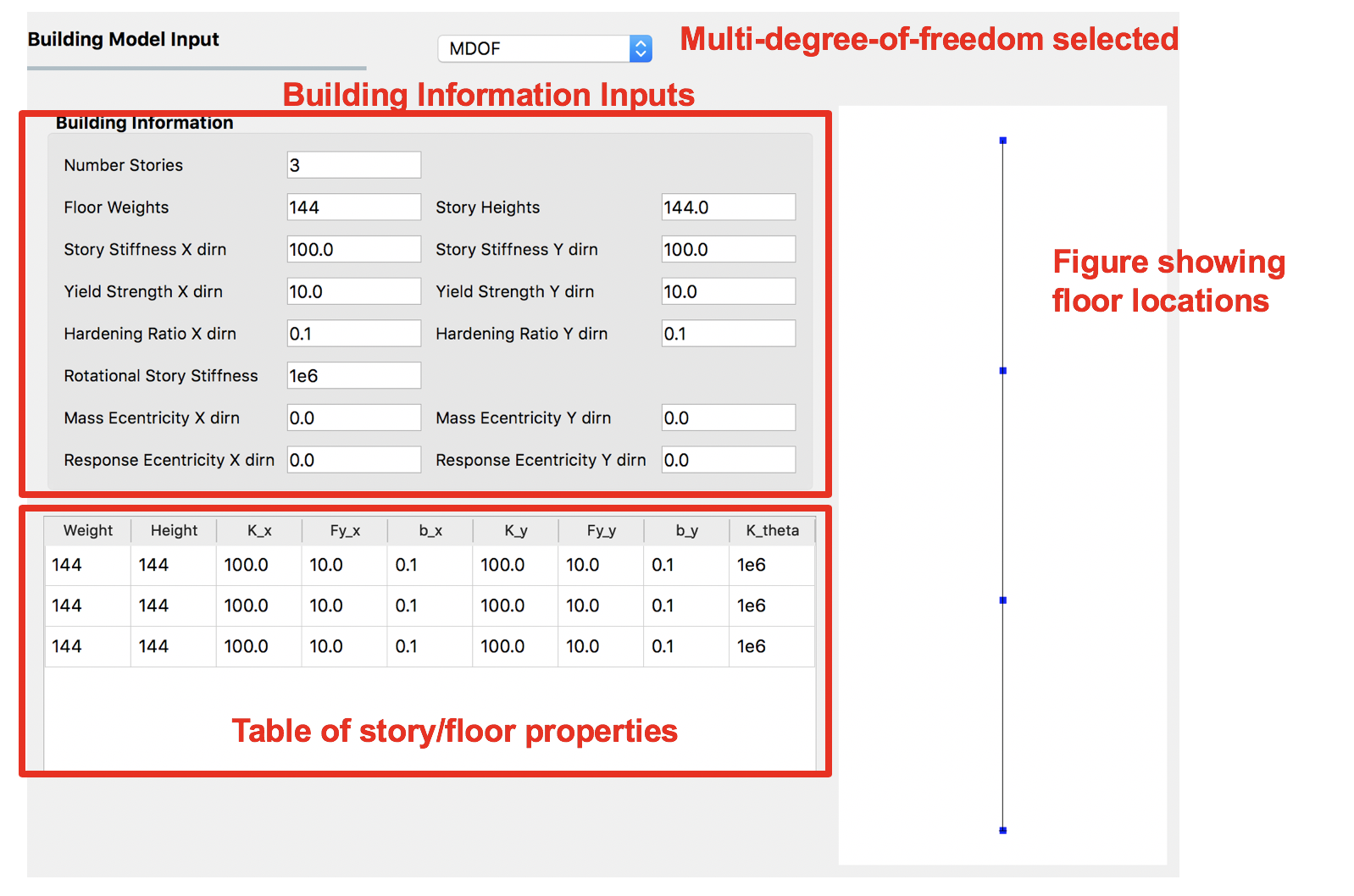
Fig. 2.3.1.1 Multiple degrees of freedom (MDOF) building model generator.
Random variables can be created by the user if they enter a valid string instead of a number in the entry fields for any entry except for the Number of floors. The variable name entered will appear as a random variable in the RV panel; it is there that the user must specify the distribution associated with the random variable.
2.3.2. OpenSees
This panel is for users who have an existing OpenSees model of a building that performs a gravity analysis and now they wish to subject that building model to one of the EVT options provided. The input panel for this option is shown in Fig. 2.3.2.1. Users need to provide three pieces of information:
Main OpenSees Script: The main script that contains the building model. This script should build a model and perform any gravity analysis of the building that is required before the event is applied.
Response Nodes: A list of node numbers that define a column line of interest for which the responses will be determined. The column nodes should be in order from ground floor to roof. The EDP workflow application uses this information to determine nodes at which displacement, acceleration, and story drifts are calculated.
An entry for the dimension of the model (i.e., 2D or 3D). This information is used when loads are applied.
Entry for the number of degrees of freedom at each node in the model.
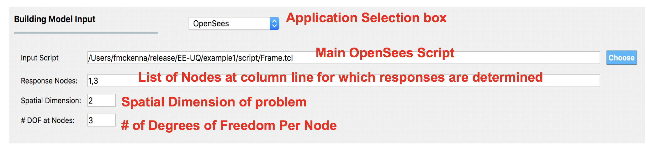
Fig. 2.3.2.1 OpenSees Model.
In OpenSees there is an option to set a variable to have a certain value using either the set or pset command, e.g pset a 5.0 will set the variable a to have a value 5 in the OpenSees script. In HydroUQ, any variable found in the main script to be set using the pset command will be assumed to be a random variable. As such, when a new main script is loaded, all variables set with pset will appear as random variables in the UQ panel.
2.3.6. MDOF-LU Building Model
The MDOF-LU building modeling application creates a hysteretic, multi-degree of freedom (MDOF) model based on the Lu method. As seen in Fig. 2.3.6.1, the following inputs are required:
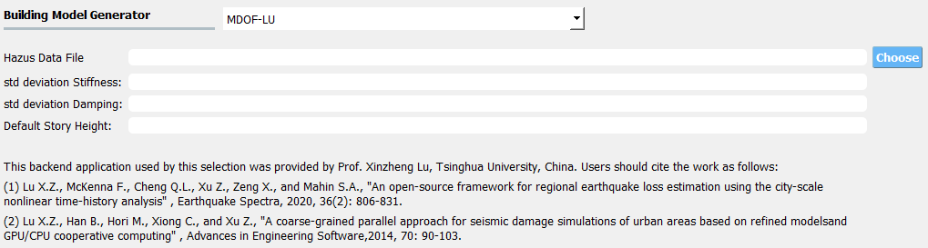
Fig. 2.3.6.1 MDOF-LU Building model input panel.
Hazus Data File: The path to a file that contains the ruleset that maps the design code-level & structural types to various structural parameters.
Hereis an example file, where the columns are in the order ofColumn names of HazusData.txt (click)
Table 2.3.6.1 Column names of HazusData.txt (showing the first 10 rows for high-code) id
str type
min #story
max #story
height
Sy
eta
C
gamma
eta_soft
alpha
beta
a_k
omega
damage1
damage2
damage3
damage4
T1
T2
hos
damp
1
W1
1
50
18.4547
0.4
0.0870354
1000
0.8
-0.001
3
1
0.1
0.2
0.004
0.012
0.04
0.1
0.35
0.33333
4.27
0.1
2
W2
1
50
56.243
0.4
0.0794118
1000
0.6
-0.001
2.5
1
0.1
0.2
0.004
0.012
0.04
0.1
0.2
0.33333
3.66
0.1
3
S1L
1
3
38.7247
0.25
0.0865974
1000
1
-0.001
3
1
0
0.2
0.006
0.012
0.03
0.08
0.25
0.33333
3.66
0.05
4
S1M
4
7
51.7562
0.156
0.133734
1000
1
-0.001
3
1
0
0.2
0.004
0.008
0.02
0.0533
0.216
0.33333
3.66
0.05
5
S1H
8
50
62.9659
0.098
0.181032
1000
1
-0.001
3
1
0
0.2
0.003
0.006
0.015
0.04
0.17
0.33333
3.66
0.05
6
S2L
1
3
56.243
0.4
0.0670927
1000
0.5
-0.001
2
1
0
0.2
0.005
0.01
0.03
0.08
0.2
0.33333
3.66
0.05
7
S2M
4
7
75.8694
0.333
0.103936
1000
0.5
-0.001
2
1
0
0.2
0.0033
0.0067
0.02
0.0533
0.172
0.33333
3.66
0.05
8
S2H
8
50
85.0452
0.254
0.142936
1000
0.5
-0.001
2
1
0
0.2
0.0025
0.005
0.015
0.04
0.136154
0.33333
3.66
0.05
9
S3
1
50
14.0607
0.4
0.0670927
1000
1
-0.001
2
1
0
0.2
0.004
0.008
0.024
0.07
0.4
0.33333
4.57
0.05
10
S4L
1
3
74.5959
0.32
0.0727412
1000
0.5
-0.001
2.25
1
0
0.2
0.004
0.008
0.024
0.07
0.175
0.33333
3.66
0.05
See Fig. 2.3.6.2 for the parameter definitions. Note that not all the parameters are being used.
Std deviation Stiffness: The standard deviation of lateral stiffness of the building model. The randomness will be applied by sampling a multiplication factor with the specified standard deviation and mean of 1. The factor is sampled only once per structure and will be applied to all stories.
Std deviation Damping: The standard deviation of the damping ratio of the building model. The randomness will be applied by sampling a multiplication factor with the specified standard deviation and mean of 1.
Default Story Height (optional): Used to set the mass node coordinates.
Once the analysis is done, the estimated structural parameters are written in SAM.json and the corresponding opensees model is written in example.tcl (with uniaxialMaterial Hysteretic material model) for the downstream analysis. Both files can be found in the local working directory.
Example of SAM.json (click)
{
    "Properties":
    {
        "dampingRatio": 0.09956333887469665,
        "uniaxialMaterials":
        [
            {
                "name": 1,
                "type": "shear",
                "K0": 61532397.052015901,
                "Sy": 2110124.6849974156,
                "eta": 0.087035399999999999,
                "C": 1000.0,
                "gamma": 0.80000000000000004,
                "alpha": 3.0,
                "beta": 1.0,
                "omega": 0.20000000000000001,
                "eta_soft": -0.001,
                "a_k": 0.10000000000000001
            },
            {
                "name": 2,
                "type": "shear",
                "K0": 61532397.052015901,
                "Sy": 1406749.7899982773,
                "eta": 0.087035399999999999,
                "C": 1000.0,
                "gamma": 0.80000000000000004,
                "alpha": 3.0,
                "beta": 1.0,
                "omega": 0.20000000000000001,
                "eta_soft": -0.001,
                "a_k": 0.10000000000000001
            }
        ]
    },
    "Geometry":
    {
        "nodes":
        [
            {
                "name": 1,
                "crd":
                [
                    0.0,
                    0.0,
                    0.0
                ],
                "ndf": 6,
                "constraints":
                [
                    1,
                    1,
                    1,
                    1,
                    1,
                    1
                ]
            },
            {
                "name": 2,
                "mass": 284190.39936000004,
                "crd":
                [
                    0.0,
                    0.0,
                    3.6000000000000001
                ],
                "ndf": 6,
                "constraints":
                [
                    0,
                    0,
                    1,
                    1,
                    1,
                    1
                ]
            },
            {
                "name": 3,
                "mass": 284190.39936000004,
                "crd":
                [
                    0.0,
                    0.0,
                    7.2000000000000002
                ],
                "ndf": 6,
                "constraints":
                [
                    0,
                    0,
                    1,
                    1,
                    1,
                    1
                ]
            }
        ],
        "elements":
        [
            {
                "name": 1,
                "type": "shear_beam2d",
                "uniaxial_material": 1,
                "nodes":
                [
                    1,
                    2
                ]
            },
            {
                "name": 2,
                "type": "shear_beam2d",
                "uniaxial_material": 2,
                "nodes":
                [
                    2,
                    3
                ]
            }
        ]
    },
    "NodeMapping":
    [
        {
            "cline": "response",
            "floor": "0",
            "node": 1
        },
        {
            "cline": "response",
            "floor": "1",
            "node": 2
        },
        {
            "cline": "response",
            "floor": "2",
            "node": 3
        }
    ],
    "units":
    {
        "force": "kN",
        "length": "m",
        "temperature": "C",
        "time": "sec"
    }
}
Example of opensees.tcl (click)
model BasicBuilder -ndm 3 -ndf 6
node 1 0 0 0
fix 1 1 1 1 1 1 1
node 2 0 0 3.6 -mass 284190 284190  0.0  0.0  0.0 2.8419e-05
fix 2 0 0 1 1 1 1
node 3 0 0 7.2 -mass 284190 284190  0.0  0.0  0.0 2.8419e-05
fix 3 0 0 1 1 1 1
uniaxialMaterial Hysteretic 1 2.11012e+06 0.0342929 6.33037e+06 0.822315 6.33037e+06 1 -2.11012e+06 -0.0342929 -6.33037e+06 -0.822315 -6.33037e+06 -1 0.8 0.8 0 0 0.1
uniaxialMaterial Hysteretic 2 1.40675e+06 0.0228619 4.22025e+06 0.54821 4.22025e+06 1 -1.40675e+06 -0.0228619 -4.22025e+06 -0.54821 -4.22025e+06 -1 0.8 0.8 0 0 0.1
element zeroLength 1 1 2 -mat 1 1 -dir 1 2
element zeroLength 2 2 3 -mat 2 2 -dir 1 2
loadConst -time 0.0
#timeSeries Path 101 -dt 0.005 -factor [expr 1 * 1 * 1 ] -values { -1.46509e-05 8.24738e-06 -2.26001e-05 1.46955e-05 -2.63045e-05 ..... -3.42224e-05  }
#timeSeries Path 102 -dt 0.005 -factor [expr 1 * 1 * 1 ] -values { 7.15223e-06 -2.4271e-05 1.94678e-05 -3.62861e-05 2.96503e-05 ...... -0.000675427  }
pattern UniformExcitation 101 1 -fact 1 -accel 101
set numStep 60000
set dt 0.005
pattern UniformExcitation 102 2 -fact 1 -accel 102
set numStep 60000
set dt 0.005
set numberOfStories 2
recorder EnvelopeNode -file 1-AIM.json0.max_abs_acceleration.response.0.out -timeSeries 101 102  -node 1 -dof 1 2  accel
recorder EnvelopeNode -file 1-AIM.json0.max_abs_acceleration.response.1.out -timeSeries 101 102  -node 2 -dof 1 2  accel
recorder EnvelopeNode -file 1-AIM.json0.max_rel_disp.response.1.out -node 2 -dof 1 2  disp
recorder EnvelopeDrift -file 1-AIM.json0.max_drift.response.0.1.1.out -iNode 1 -jNode 2 -dof 1 -perpDirn 3
recorder EnvelopeDrift -file 1-AIM.json0.max_drift.response.0.1.2.out -iNode 1 -jNode 2 -dof 2 -perpDirn 3
recorder EnvelopeNode -file 1-AIM.json0.max_abs_acceleration.response.2.out -timeSeries 101 102  -node 3 -dof 1 2  accel
recorder EnvelopeNode -file 1-AIM.json0.max_rel_disp.response.2.out -node 3 -dof 1 2  disp
recorder EnvelopeDrift -file 1-AIM.json0.max_drift.response.1.2.1.out -iNode 2 -jNode 3 -dof 1 -perpDirn 3
recorder EnvelopeDrift -file 1-AIM.json0.max_drift.response.1.2.2.out -iNode 2 -jNode 3 -dof 2 -perpDirn 3
recorder EnvelopeDrift -file 1-AIM.json0.max_roof_drift.response.0.2.1.out -iNode 1 -jNode 3 -dof 1 -perpDirn 3
recorder EnvelopeDrift -file 1-AIM.json0.max_roof_drift.response.0.2.2.out -iNode 1 -jNode 3 -dof 2 -perpDirn 3

# Perform the analysis
numberer RCM
constraints Transformation
system Umfpack
integrator Newmark 0.5 0.25
test NormUnbalance 1.0e-2 10
algorithm Newton
analysis Transient -numSubLevels 2 -numSubSteps 10
set xDamp 0.0995633;
set lambdaN [eigen 3];
set lambdaI [lindex $lambdaN [expr 1 -1]];
set lambdaJ [lindex $lambdaN [expr 3 -1]];
set lambda1 [lindex $lambdaN 0]
set omega1 [expr pow($lambda1,0.5)];
set omegaI [expr pow($lambdaI,0.5)];
set omegaJ [expr pow($lambdaJ,0.5)];
set alphaM [expr $xDamp*(2*$omegaI*$omegaJ)/($omegaI+$omegaJ)];
set betaKinit [expr 0 *2.0*$xDamp/($omegaI+$omegaJ)];
set betaKcomm [expr 0 *2.0*$xDamp/($omegaI+$omegaJ)];
set betaKcurr [expr 1 *2.0*$xDamp/($omegaI+$omegaJ)];
rayleigh $alphaM $betaKcurr $betaKinit $betaKcomm;
set lambdaN [eigen 1];
set lambda1 [lindex $lambdaN 0]
set T1 [expr 2*3.14159/$lambda1]
set dTana [expr $T1/20.]
if {$dt < $dTana} {set dTana $dt}
analyze [expr int($numStep*$dt/$dTana)] $dTana
remove recorders
where the keys of SAM.json are defined as follows:
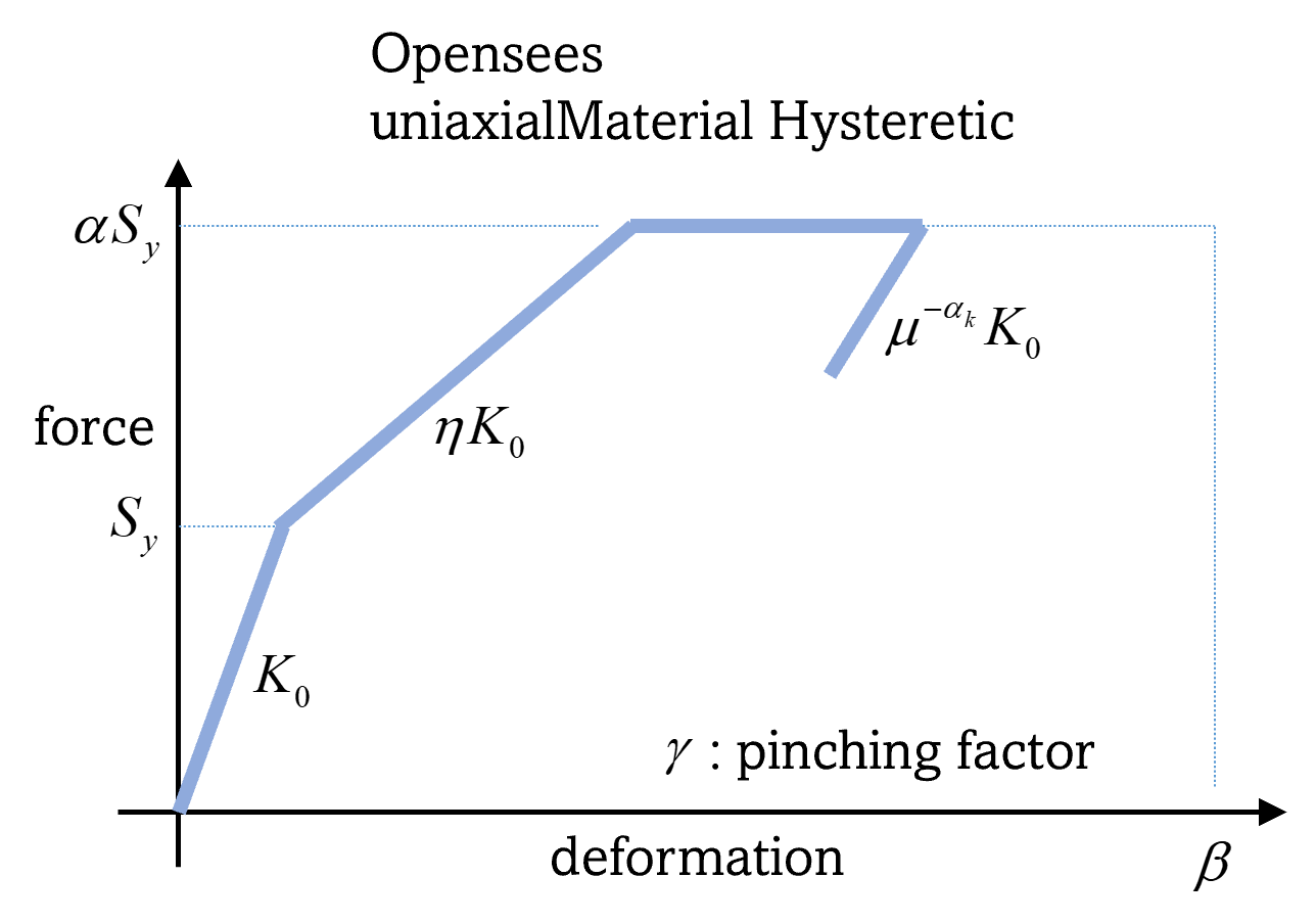
Fig. 2.3.6.2 MDOF-LU Building model.
Note
When the MDOF-LU building modeling application is employed, the OpenSees simulation application should be used for analysis in the ANA: Asset Analysis input panel.
Lu, X., McKenna, F., Cheng, Q., Xu, Z., Zeng, X., & Mahin, S. A. (2020). An open-source framework for regional earthquake loss estimation using the city-scale nonlinear time history analysis. Earthquake Spectra, 36(2), 806-831.
2.3.7. Multiple Models
The Multiple Models structural modeling application allows users to define multiple structural models for use in their analysis. The Add and Remove buttons allow users to control the number of models they want to use in the analysis.
By adding a model, a new tab is created in the SIM panel where users can choose one of the structural modeling applications described in the sections above and provide the inputs necessary to create the model. Users also need to specify their belief about the credibility of the model in the tab corresponding to that model. The beliefs are expressed as non-negative numerical values. The belief value for each model is defined relative to the other models, and the beliefs do not need to sum to 1.
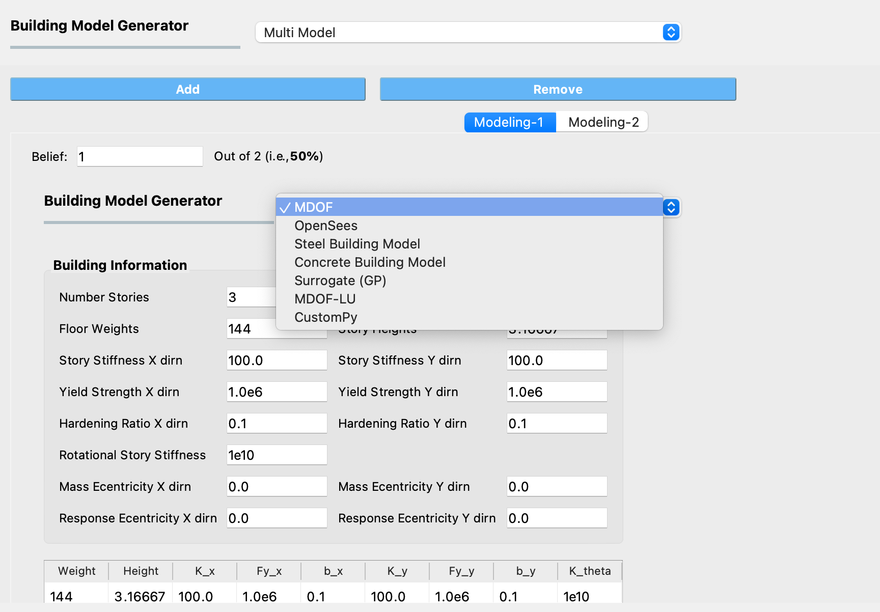
Fig. 2.3.7.1 Selecting a structural modeling application within a Multiple Models SIM Application
Note
If a Multiple Models application is selected, at least 2 models must be defined.
Note
If the “Multi-fidelity Monte Carlo (MFMC)” option was selected in the UQ tab, the belief values will be ignored. The premise of MFMC is that the high-fidelity model response always provides the best response, therefore, the conception of belief does not apply.