4.1. Stochastically Generated Wind Loading

The purpose of this analysis is to verify that WE-UQ app is able to reproduce the correct power spectral density when using stochastically generated wind speed time histories. These time histories are generated using a discrete frequency function and Fast Fourier Transform, as described in Wittig & Sinha (1975) [WS75]. The calculated power spectral density matrix for the generated time histories is compared to an analytical spectral density matrix based on the Kaimal wind spectrum model [KWICote72, SS96] and the Davenport coherence function [Dav67]:

(4.1.1)\[S_{rs} = \sqrt{S_{rr}(f) \cdot S_{ss}(f)} Coh(f)\]

where :math`S_{rr}` and \(S_{ss}\) are power spectral densities of fluctuating wind at locations \(r\) and \(s\) respectively; \(Coh(f)\) is the Davenport coherence function; and \(f\) is the frequency in Hz. This gives the two-dimensional, \(n\)-variate power spectral density matrix \(S(f)\):

(4.1.2)\[\begin{split}S(f) = \begin{bmatrix} S_{11}(f) & S_{12}(f) & \dots & S_{1n}(f) \\ S_{21}(f) & S_{12}(f) & \dots & S_{2n}(f) \\ \vdots & \vdots & \ddots & \vdots \\ S_{n1}(f) & S_{n2}(f) & \dots & S_{nn}(f) \\ \end{bmatrix}\end{split}\]

The power spectral density based on the Kaimal wind spectrum is defined as:

(4.1.3)\[S_{rr}(z_{r}, f) = u_{*}^{2} \cdot \frac{200 z_{r}}{\bar{U}(z_{r})} \cdot \frac{1}{\left[1 + 50 \frac{f z_{r}}{\bar{U}(z_{r})}\right]^{\frac{5}{3}}}\]

where \(S_{rr}(f)\) is the power spectral density of the fluctuating wind at location \(z_{r}\) and frequency \(f\) in Hz; \(\bar{U}(z_{r})\) is the mean wind speed at location \(z_{r}\); and \(u_{*}\) is the friction velocity. The one-sided Davenport coherence function describes the correlation between fluctuating winds at locations \(z_{r}\) and \(z_{s}\):

(4.1.4)\[Coh(f) = \text{exp}\left[-\frac{C_{z}f\lvert z_{r} - z_{s}\rvert}{\frac{1}{2}\left[\bar{U}(z_{r}) + \bar{U}(z_{s})\right]}\right]\]

The mean wind velocity at location \(z_{r}\) is defined based on exposure conditions defined in the ASCE 7 standard as follows:

(4.1.5)\[\bar{U}(z) = \bar{b} \left(\frac{z}{33}\right)^{\bar{\alpha}}\left(\frac{88}{60}\right)V\]

where \(\bar{b}\) and \(\bar{\alpha}\) are constants defined in ASCE 7 for different exposure conditions; \(V\) is the 3-second gust wind speed in miles per hour.

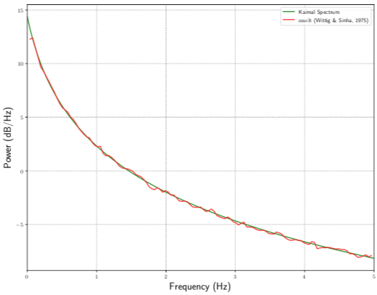
Fig. 4.1.2 Comparison between theoretical and simulated auto power spectral density at the height of the first floor

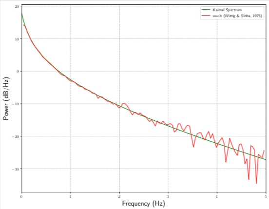
Fig. 4.1.3 Comparison between theoretical and simulated cross power spectral density between the heights of the second and third floors

In the validation example, a 3-story structure with exposure category D is subjected to wind loading with 3-second gust of 30 mph. An estimate of the power spectral density matrix for the stochastic wind velocity time history based on this condition was compared to the power spectral density matrix calculated based on the Kaimal spectrum with Davenport coherence. Fig. 4.1.2 shows the auto correlation for the first floor (\(S_{11}\)) while Fig. 4.1.3 shows the cross correlation between the second and third floors (\(S_{23}\)). As can be seen in these two figures, the two different results show very good agreement between the theoretical Kaimal values and the estimates based on the generated stochastic wind velocity time histories. Further information on the implementation of the Wittig & Sinha (1975) model can be found in the documentation for smelt a C++ library for stochastically generating time histories for different types of natural hazards.