2.4.5. Site Response Analysis¶

s³hark allows users to determine the event at the base of the building by performing an effective free-field site response analysis of a soil column. In this panel, the user specifies a ground motion at the bottom of the soil column. After the soil layers have been properly defined, the motion at the ground surface is given at the end of the analysis and that motion can be used in the simulation of the building response.

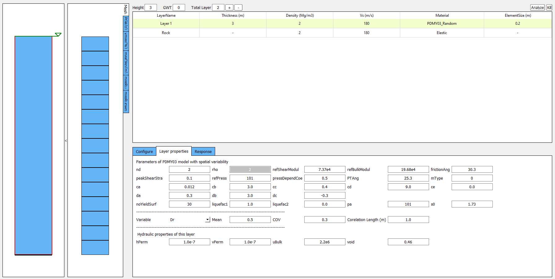
The full user graphic interface looks like what is shown in Fig. 2.4.5.1

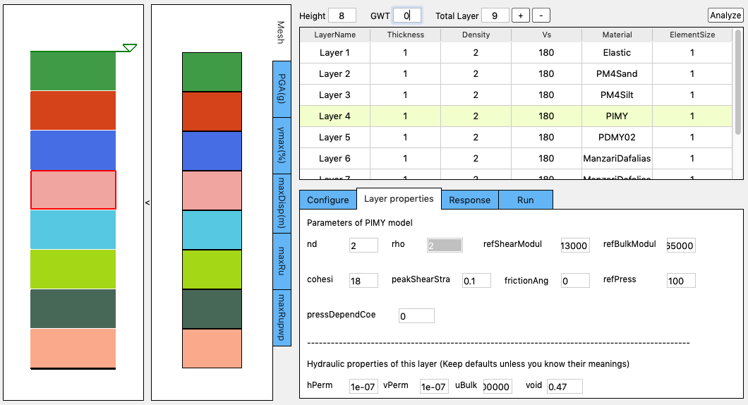
Fig. 2.4.5.1 Full Graphic Interface¶

Clicking the arrow between the Soil Column Graphic and the FE Mesh Graphic will hide the FE Mesh Graphic, which makes the UI look like what is shown in Fig. 2.4.5.2.

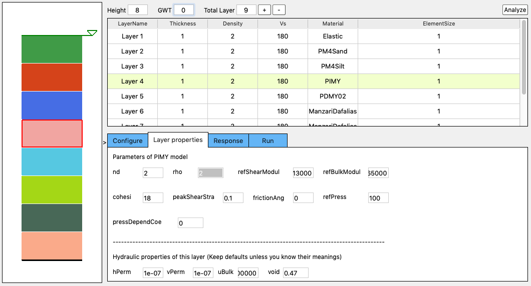
Fig. 2.4.5.2 Collapse Graphic Interface¶

The UI of s³hark consists of the following components:

2.4.5.1. Soil Column Graphic¶

The first graphic on the left of the panel shows a visualization of the soil column created. Each layer has a different randomly generated color. When the user adds or deletes a soil layer, this graphic will refresh.

2.4.5.2. FE Mesh Graphic¶

The second graphic on the left shows the finite element mesh and profile plots. Upon the finish of the analysis, select any of the tabs on the right inside this graphic (i.e., PGA, $γ m a x$ , maxDisp, maxRu, maxRuPWP) will show various results from the simulation at the mesh points.

2.4.5.3. Operations Area¶

The right side of this area shows some information on the created soil column, such as the total height and number of soil layers. The user also finds the Ground Water Table (GWT) input field, plus and minus buttons in this area. If the user presses the plus button, a layer will be added below a currently selected layer. If the minus button is pressed the currently selected layer will be removed. The GWT input field allows the user to specify the level of the groundwater table.

Note

Variables are assumed to have m, kPa, and kN units in s³hark.

2.4.5.4. Soil Layer Table¶

This table is where the user provides the characteristics of soil layers, such as layer thickness, density, Vs30, material type, and element size in the finite element mesh. Single click at a cell will make a soil layer, which will highlight the layer using green color in the table. Also the layer will be highlighted by a red box in the Soil Column Graphic. Meanwhile the Layer Properties Tab will be activated. Double-click a cell to edit it in the table. If you change the Material cell of a layer, the Layer Properties Tab will change correspondingly.

2.4.5.5. Tabbed Area¶

This area contains the three tabbed widgets described below.

Configure Tab¶

This tab allows the user to specify the paths to the OpenSees executable and a ground motion file that represent the ground shaking at the bedrock. The rock motion file must follow the SimCenter event format. Examples of SimCenter event files are available in the motion demos. s³hark will determine whether to use a 2D column or 3D column based on the ground motion file provided. When a ground motion file is selected from the local computer or the path of the ground motion file is typed in, s³hark will figure out if it’s a 1D or 2D shaking file. If it’s 1D shaking, all elements will be 2D. If it’s 2D shaking, all elements will be 3D. The definitions of 2D and 3D slope are different. See Fig. 2.4.5.8.2 and Fig. 2.4.5.8.4.

More details about this tab can be found in Configure.

Layer Properties Tab¶

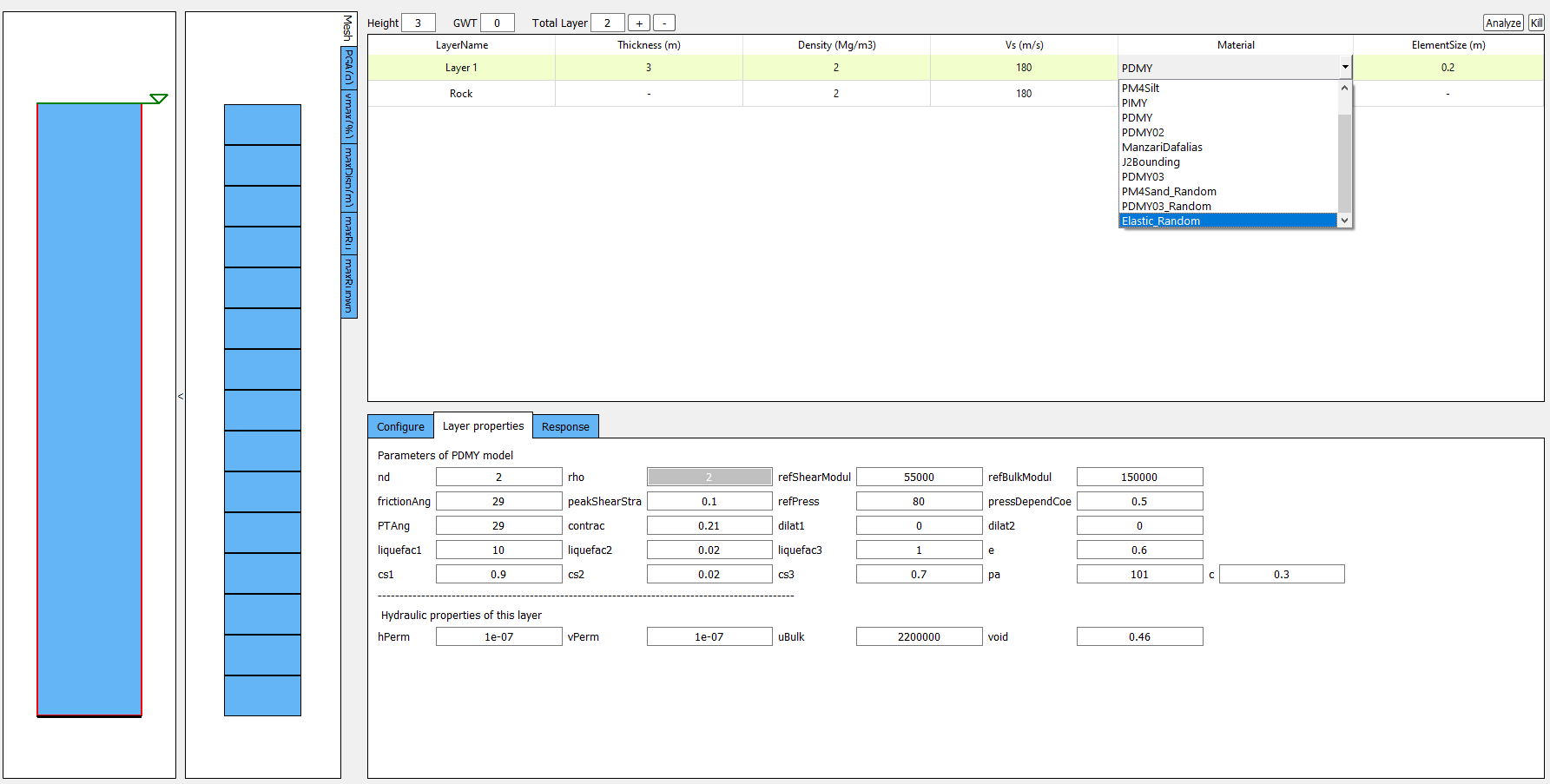
This tab allows the user to enter additional material properties for the selected soil layer Fig. 2.4.5.5.1.

Fig. 2.4.5.5.1 Layer properties¶

Response Tab¶

Once the site response analysis has been performed, this tab provides information about element and nodal time varying response quantities. See Fig. 2.4.5.5.2.

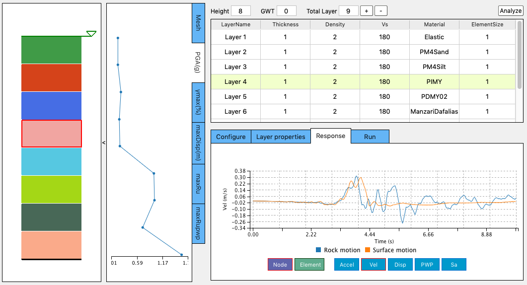
Fig. 2.4.5.5.2 Response¶

2.4.5.6. Analyze Button¶

This Analyze button is located at the top-right corner of the UI and shall be used to run the simulation locally on your computer. A progress bar will show up at the bottom of the application indicating the status of the analysis. Upon the finish of the simulation, a message will be displayed (Fig. 2.4.5.6.1).

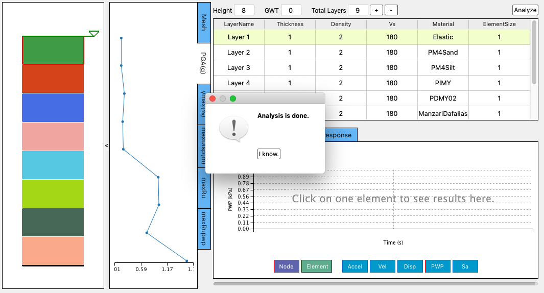
Fig. 2.4.5.6.1 Analysis is done¶

2.4.5.7. View Results¶

Click the button to dismiss the message window, the response tab will be activated. The user can click on any element in the mesh graphic, the selected element will be highlighted in red and the selected nodes will be pointed out by blue arrows. The time history of the selected element/node will be shown in the Response Tab. This allows the user to review the ground motion predicted at selected nodes Fig. 2.4.5.7.1.

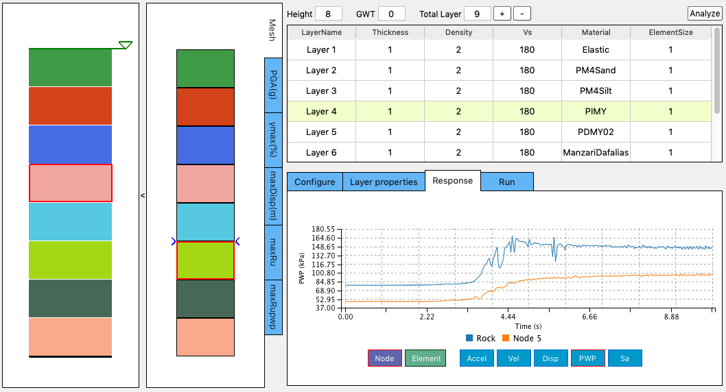
Fig. 2.4.5.7.1 Response at a selected node¶

Note

If the Analyze button is not pressed, no simulation will be performed, therefore no simulation is performed and there will be no ground motions provided to the building if you are using s³hark inside other SimCenter applications.

2.4.5.8. Configure¶

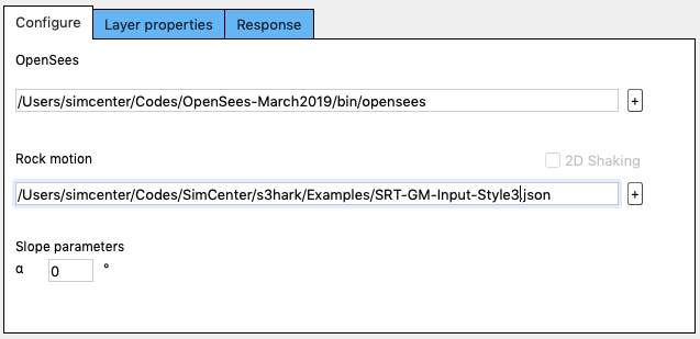
Fig. 2.4.5.8.1 Configuration with a 1D shaking motion¶

In the configure tab, two paths need to be specified. You can either type them or click the ‘+’ button to select them from your computer. If you don’t have OpenSees installed, the instruction can be found here. If you don’t have a ground motion file, demos can be downloaded here.

Note

Variables are assumed to have m, kPa, and kN units in s³hark.

The first demo is SRT-GM-Input-Style3.json, which contains the shaking motion in one direction (1D shaking). If you select this file as the input motion, your tab will look like the one shown in Fig. 2.4.5.8.1. You can edit the slope degree $α$ . For flat ground, the value should be set as 0. If 1D shaking motion provided, s³hark automatically treats the problem as a 2D plane strain problem. 2D elements will be used. The slope diagram is plotted in Fig. 2.4.5.8.2.

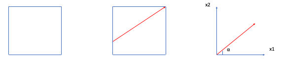
Fig. 2.4.5.8.2 Slope definition for 2D Column¶

The second demo is SRT-GM-Input-Style3-2D.json, which contains the shaking motion in two directions (2D shaking). If you select this file as the input motion, your tab will look like the one shown in Fig. 2.4.5.8.3.

Fig. 2.4.5.8.3 Configuration with a bi-directional shaking motion¶

You can see s³hark detected the file you provided is a 2D shaking, s³hark automatically treats the problem as a 3D problem. 3D elements will be used. The slope diagram is plotted in Fig. 2.4.5.8.4:

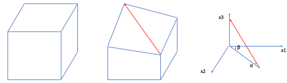
Fig. 2.4.5.8.4 Slope definition for 3D Column¶

For flat ground $α$ and $β$ should be set as 0.

2.4.5.9. Modeling Spatial Variability Uncertainty of Soil¶

The most recent version of s³hark allows the user to include spatial variability in the definition of soil profile. This functionality is achieved using several newly added SimCenter backend python scripts.

Generating Gaussian Random field¶

Physical properties of soils vary from place to place within a soil deposit due to varying geologic formation and loading histories such as sedimentation, erosion, transportation, and weathering processes. This spatial variability in the soil properties cannot be simply described by a mean and variance since the estimation of the two statistic values does not account for the spatial variation of the soil property data in the soil profile. Spatial variability is often modeled using two separated components: a known deterministic trend and a residual variability about the trend. These components are illustrated in Fig. 2.4.5.9.1.

../../../../../_images/InherentVariability1.png

Fig. 2.4.5.9.1 Inherent soil variability (after [PK99]).¶

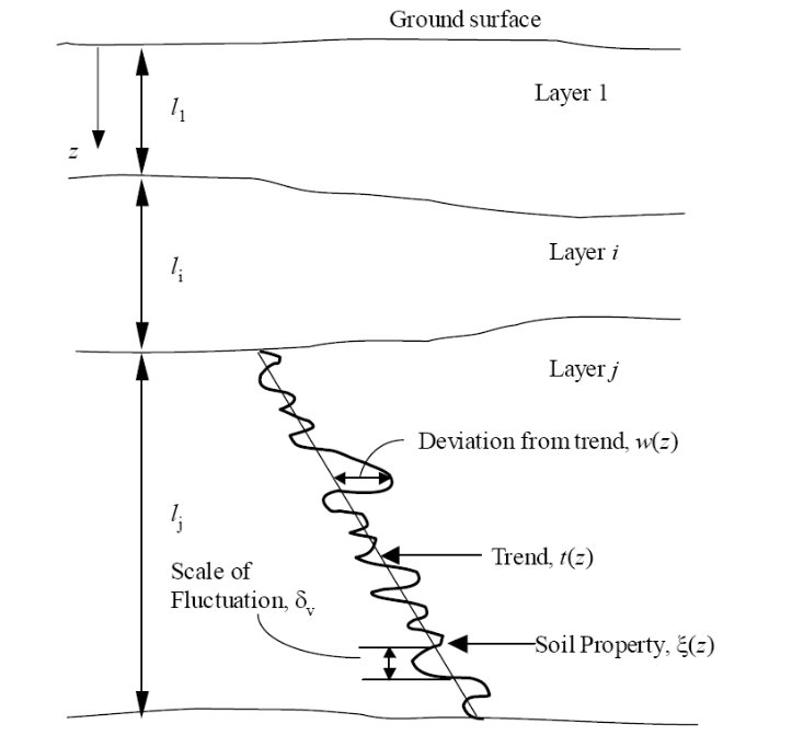
This simplified spatial variability proposed by [PK99] can be expressed as,

(2.4.5.9.1)¶

ξ (z) = t (z) + w (z),

where $ξ (z)$ = soil property at location $z$ , $t (z)$ = deterministic trend at $z$ , and $w (z)$ = residual variation. The trend is a smooth deterministic function that can be obtained from a regression analysis of measured data. The residuals are characterized statistically as random variables, usually with zero mean and non-zero variance. The pattern of the residuals depends on the local spatial variability of a property. The residual about a trend does not change erratically in a probabilistically independent way. Rather, similar property values (positive or negative residuals around a trend) occur together in adjacent locations characterizing the scale of fluctuation (or wavelength of a residual along the trend) as shown in Fig. 2.4.5.9.1.

Gaussian stochastic random fields are generated for the liquefiable soil layer by randomizing the assigned soil strength parameter over the soil layers with a certain spatial probability density. [Shi07] introduced a procedure for generating stochastic random field based on the method outlined in [YS88] considering uncertainties in soil properties. As explained earlier, the stochastic random field for a soil property consists of a trend (or mean) field and a residual field,

(2.4.5.9.2)¶

F_{s t o c h a s t i c} = F_{t r e n d} + F_{r e s i d u a l} .

The trend field ( $t (z)$ ) represents the deterministic mean field assigned by the user. To obtain the residual field ( $w (z)$ ), a Gaussian random field can be generated using the algorithm proposed by [YS88]. A normal distribution with a coefficient of variation, COV, is required. The scale of fluctuation is defined by correlation length. The values obtained using [YS88]’s method are interpolated according to the soil element center locations.

A summary of the random field preparation procedure for the site response event analysis is summarized here: Enumerated lists:

Generate mean field using mean target soil property, e.g., relative density or shear wave velocity
Generate Gaussian random field for target soil property using Gauss1D.py with mean = 0.0 and $σ$ = 1.0
Interpolate Gaussian field to FEM mesh
Combine the mean field and Gaussian field to obtain a stochastic field using the following equation:

(2.4.5.9.3)¶

F_{s t o c h a s t i c} = F_{m e a n} + F_{r e s i d u a l} = F_{m e a n} + C O V F_{m e a n} F_{G a u s s i a n}

Note

A reasonable mesh resolution is recommended. The selection of element size should consider several factors, including but not limited to, layer shear wave velocity (for frequency resolution), correlation length (for random field resolution), and computation efficiency.

Calibration of Constitutive Model¶

Since soil properties, instead of material input parameters, are randomized, it is imperative to choose representative input parameters for constitutive models based on the random variable chosen by the user. An independent calibration process of the constitutive model should be carried out carefully. Currently, a couple of pre-calibrated correlations are included in s³hark, including PM4Sand and PDMY03 based on relative density ( $D_{R}$ ). The detailed correlation can be found in calibration.py. The user is also encouraged to modify the script to include their own calibration of constitutive models.

Currently, three constitutive models are supported in s³hark to have random fields, namely, Elastic Isotropic (Elastic_Random), PM4Sand (PM4Sand_Random), and PDMY03 (PDMY03_Random). When these models are selected, the analysis will be carried out using SimCenter workflow. As a result, profile and response plots are not updated inside s³hark.

Note

Currently only 2D plain-strain materials (including PDMY03 and ElasticIsotropic) are supported when using random field. Therefore, 1-component motion is required.

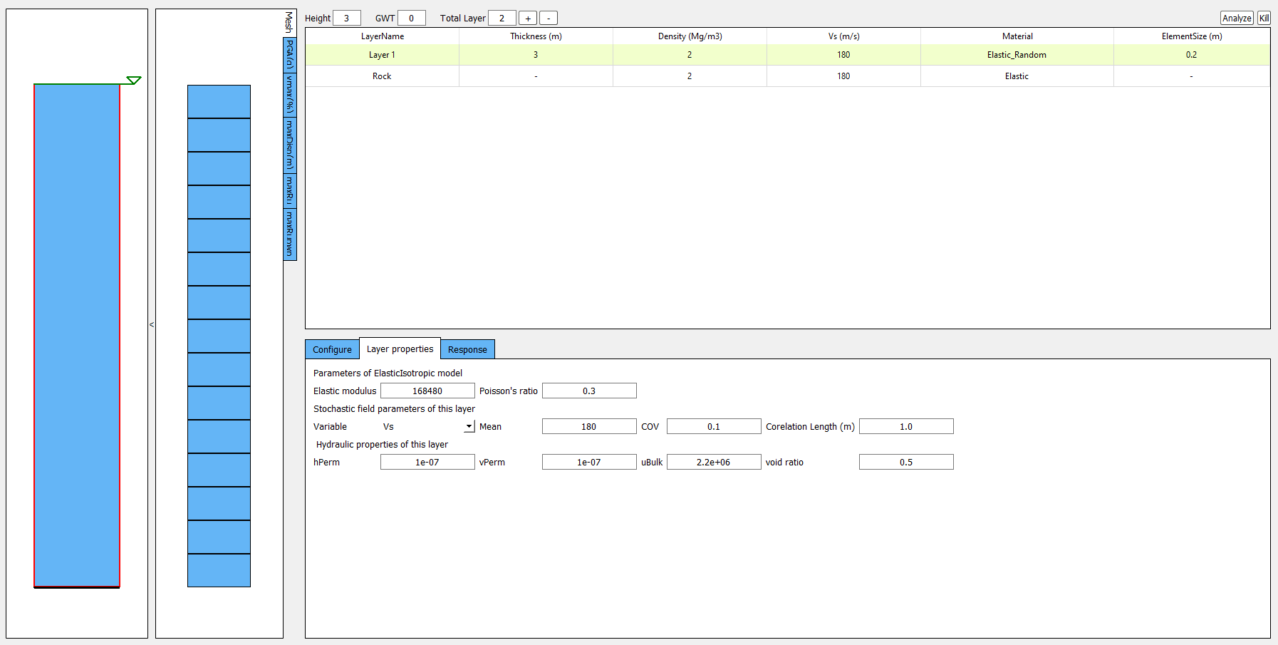
Elastic Isotropic¶

Shear wave velocity (Vs) can be selected to be randomized for this material. Subsequently, Young’s modulus is calculated based the stochastic shear velocity profile at the center of each element. No special calibration is required.

../../../../../_images/Elastic_Random.png

Note

Vs is bounded between 50 and 1500 m/s in calibration.py

PM4Sand¶

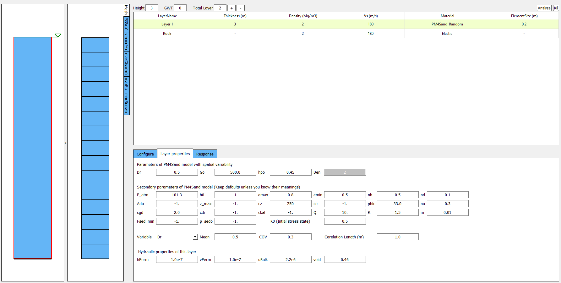
The calibration of the PM4Sand model is based on a parametric study using quoFEM [CA20]. The calibration procedure for PM4Sand is straightforward for general sand-like soil behaviors as intended by the model developers. When detailed laboratory test results are available, the apparent relative density $D_{R}$ can be estimated using void ratio and measured $e_{m a x}$ and $e_{m i n}$ . However, as discussed in [BZ15], $D_{R}$ is defined to bound the model response rather than a strict measured of relative density from maximum and minimum density tests. Therefore, the user can adjust its value as part of the calibration process, and the default critical state line might need to be re-positioned by adjusting secondary parameters $Q$ and $R$ , as well. Nevertheless, the estimated $D_{R}$ provides a reasonable value, such that the resulting model response is also reasonable. $G_{o}$ can be estimated using small-strain shear modulus estimation methods for different confining pressures. Once $D_{R}$ and $G_{o}$ are determined, $h_{p o}$ can be calibrated iteratively by matching: 1) excess pore pressure evolution for a range of individual laboratory tests, and/or 2) specific values of $C R R$ . Additional secondary parameters can also be adjusted to fine-tune the model response. For example, adjusting $h_{o}$ can result in different modulus reduction curves.

On the other hand, when comprehensive laboratory tests are not available for specific sites, model calibration needs to be based on in-situ test data such as SPT blow count, CPT penetration resistance, or shear wave velocity (Vs). For example, $D_{R}$ can be estimated by correlations to penetration resistances. [IB08] recommended the following correlation to SPT,

(2.4.5.9.4)¶

D_{R} = \sqrt{\frac{(N_{1})_{60}}{C_{d}}},

where $C_{d}$ is recommended to be 46. For CPT, the following correlation can be used,

(2.4.5.9.5)¶

D_{R} = 0.465 (\frac{q_{c 1 N}}{C_{d q}})^{0.264} - 1.063,

where $C_{d q}$ is recommended to be 0.9. The second primary input parameter $G_{o}$ can also be estimated from in-situ data. [BZ15] modified the correlation by [AS00] to constraint the extrapolation to very small $(N_{1})_{60}$ values, as

(2.4.5.9.6)¶

V_{s 1} = 85 [(N_{1})_{60} + 2.5]^{0.25} .

Alternatively, a simpler expression can be used when combined with a range of typical densities as,

(2.4.5.9.7)¶

G_{o} = 167 \sqrt{(N_{1})_{60} + 2.5} .

Subsequently, $h_{p o}$ can be calibrated to reproduce a specific value of $C R R$ that can be computed using liquefaction triggering models. Numerous liquefaction triggering models incorporating the simplified cyclic stress approach have been proposed in the past such as [YI01], [CTH+04], and [IB08]. Once $D_{R}$ , $G_{o}$ , and $C R R$ are chosen, the modeler should iteratively vary the value of $h_{p o}$ until the simulated $C R R$ matches the targeted value. Interpolation and extrapolation are common when the variables are within or close to the range of existing calibrated sets of parameters. Secondary parameters are less common to be modified when only in-situ data are available. This calibration process can become cumbersome when in-situ data show a large degree of variability and calibration has to be performed for each soil unit. To shed light on the calibration process under this circumstance, a parametric study was conducted to establish a correlation among $D_{R}$ , $G_{o}$ , $h_{p o}$ , and CRR, i.e., $C R R = f (D_{R}, G_{o}, h_{p o})$ . The function, $f$ , should be solvable for $h_{p o}$ when the other variables are known and eventually yield $h_{p o} = g (C R R, D_{R}, G_{o})$ . This correlation is intended to provide a preliminary estimation of $h_{p o}$ and simplify the iterative calibration process under selected $D_{R}$ , $G_{o}$ , and CRR, especially when both SPT and $V_{s}$ data are available and the user wants to make $G_{o}$ independent to $D_{R}$ . For this purpose, the Dakota platform, run through the uqFEM (now quoFEM) tool was used in this parametric study. uqFEM was modified to include UW MixedDriver tool. All the simulations were performed on the Texas Advanced Computing Center (http://www.tacc.utexas.edu) Frontera supercomputer made available through DesignSafe-ci.

Using this tool, $D_{R}$ , $G_{o}$ , and $h_{p o}$ were varied while all the secondary parameters were kept of their default values (predefined by primary parameters and initial stresses). The Latin Hypercube Sampling (LHS) method was used to generate near-random variables. Each of these three variables was assigned an independent uniform distribution between minimum and maximum values. The range of these variables was chosen to cover a reasonable range of scenarios and can be extended in future studies. $D_{R}$ was set to be between 0.2 to 0.9, $G_{o}$ between $250$ to $1200$ , and $h_{p o}$ between $0.05$ to $1.2$ . A total of one million samples were generated. For each set of parameters, Dakota ran MixedDriver to simulate undrained cyclic simple shear tests for 15 different CSRs ranging from $0.05$ to $0.8$ to produce smooth cyclic strength curves. A total of three initial conditions were considered: initial effective vertical stress $σ_{v}^{'} = 1 a t m .$ with $K_{0}$ equal to 0.5 and 1.0, respectively, and $σ_{v}^{'} = 2 a t m .$ with $K_{0}$ equal to 0.5. The analyses were capped at 350 uniform cycles. Once all 15 simulated CDSS tests were done, a python script was called by Dakota to calculate the number of cycles to reach liquefaction; which was defined as the number of cycles required to reach a single amplitude (SA) shear strain of 3% as recommended by [Ish93]. Number of cycles to reach 1% and 2% SA and the slope (-b) and intercept (a) of the CSR curves ([IB08]) in logarithmic scale were also recorded. The number of cycles were rounded up to the nearest half. Then a cyclic strength curve was interpolated to calculate the Cyclic Resistance Ratio, CRR, which was determined as the CSR corresponding to 15 cycles. CRRs were bounded between 0.05 and 0.5 for interpolation accuracy.

The results were processed through linear regression analysis using Matlab to find the correlation between the input, $D_{R}$ , $h_{p o}$ and $G_{o}$ , and the output CRR. Different combinations of terms were explored and the following format produced the largest $R^{2}$ ,

(2.4.5.9.8)¶

\begin{array}{r} \begin{aligned} C R R_{3 %, K_{0} = 0.5} = & 0.1282 - 0.4952 D_{R} - 5.0565 \times 10^{- 5} G_{o} + 0.0749 h_{p o} + 1.4665 \times 10^{- 4} D_{R} G_{o} \\ + 0.1323 D_{R} h_{p o} + 0.7252 D_{R}^{2} - 0.0636 h_{p o}^{2}, \end{aligned} \end{array}

with $R^{2} = 0.989$ . In this equation $D_{R}$ is in fraction. CRRs using criteria of $1 %$ and $2 %$ SA as well as for other $σ_{v}^{'}$ and $K_{0}$ were also analyzed. More results can be found in [CA20]. It should be noted that the magnitude of these coefficients depends directly on the scale of the selected variables and smaller coefficients don’t necessary imply less important features. For example, $G_{o}$ is approximately three orders of magnitude larger than $D_{R}$ , which leads to much smaller coefficients for it.

Then this equation can be rearranged to isolate $h_{p o}$ ,

(2.4.5.9.9)¶

a h_{p o}^{2} + b h_{p o} + c = 0,

where $a = 0.0636$ , $b = - 0.0749 - 0.1323 D_{R}$ , and $c = - 0.1282 + 0.4952 D_{R} + 5.0565 \times 10^{- 5} G_{o} - 1.4665 \times 10^{- 4} D_{R} G_{o} - 0.7252 D_{R}^{2} + C R R_{3 %, K_{0} = 0.5}$ . This correlation becomes a quadratic equation for $h_{p o}$ that can be solved for two real roots for $h_{p o}$ when values of $D_{R}$ , $G_{o}$ , and $C R R$ are given. The lesser root is the one that can be paired with $D_{R}$ and $G_{o}$ to yield the desired CRR in a calibration process. The predictive equation can be used to provide good initial $h_{p o}$ values and speed up the calibration process.

Note

$D_{R}$ is bounded between 0.2 and 0.95 in calibration.py

PressureDenpendentMultiYield03¶

../../../../../_images/PDMY03_Random.png

PressureDenpendentMultiYield03 is updated from PressureDenpendentMultiYield02, which was developed for liquefaction and cyclic mobility, to comply with the established guidelines on the dependence of liquefaction triggering to the number of loading cycles, effective overburden stress ( $K σ$ ), and static shear stress ( $K α$ ). The model has been improved with new flow rules to better capture contraction and dilation in sands and has been implemented as PDMY03 in OpenSees. In s³hark, the calibration of PDMY03 model is based on interpolating pre-calibrated parameter sets for various of relative densities.

../../../../../_images/Pdmy03_parameters.png

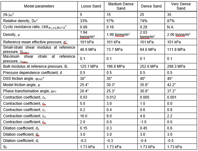
Fig. 2.4.5.9.2 Calibrated parameters for PDMY03 (after [KELL18]).¶

Note

$D_{R}$ is bounded between 0.33 and 0.87 in calibration.py