2.4.3. Stochastic Wave Loading

Sample JONSWAP sea states and compute Wheeler-corrected Morison loads on an assumed monopile-like structure. The module builds a wave power spectral density (PSD) from your inputs (e.g., significant wave height, peak period), samples a wave elevation time series at the structure site, and then evaluates vertical stacks of load recorders along the monopile. These loads are later mapped onto full structural models (e.g., in OpenSees) in the SimCenter workflow to determine structural response.

Warning

The JONSWAP spectrum was derived from North Sea field data and is conditionally applicable. It can be reasonable for North Atlantic offshore conditions (e.g., Maine/Norway) under appropriate sea states, but it is a placeholder that advanced users may replace with a more site-specific spectrum.

The implementation uses a validated Python backend (welib) for JONSWAP and Wheeler-corrected Morison loading and is designed to run quickly (tens-hundreds of samples typically complete in minutes).

2.4.3.1. GUI at a Glance

• Left column — All input parameters.

• Center plot — Wave Spectra (PSD vs Frequency). Click Sample Wave Spectra to build the JONSWAP spectrum from the current parameters.

• Right plot — Wave Time Series (Surface Displacement vs Time). Click Sample Time Series to synthesize a realization of the free-surface elevation.

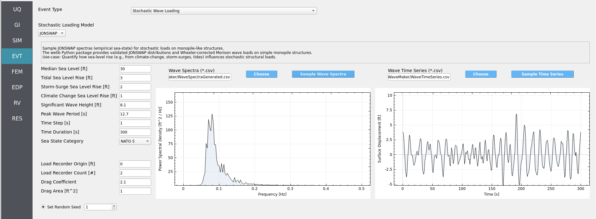
Fig. 2.4.3.1.1 Stochastic Wave Loading GUI in HydroUQ v4.2.0

2.4.3.2. Parameters

Note

Any parameter can be turned into a Random Variable by entering an alphabetic name instead of a number. Then define its distribution in the Random Variables (RV) sidebar to propagate hydrodynamic uncertainty through your workflow.

Water Level (ft)

Parameter	Description
Median Sea Level	Reference water level about which fluctuations occur.
Tidal Sea Level Rise	Tidal offset relative to the median level.
Storm-Surge Sea Level Rise	Event-based surge offset.
Climate Change Sea Level Rise	Long-term mean sea-level shift.

Sea State

Parameter	Description
Significant Wave Height (ft)	JONSWAP input height (H_s).
Peak Wave Period (s)	JONSWAP peak period (T_p).
Sea State Category [NATO 1–5]	Deprecated. Shown for legacy compatibility; prefer explicit H_s and T_p.

Deprecated since version The: Sea State Category control is legacy-only and may be removed in a future release.

Time Discretization

Parameter	Description
Time Step (s)	Sampling interval for the synthesized time series (e.g., 1.0 s).
Time Duration (s)	Total simulated duration (e.g., 300 - 3600 s).

Warning

Using an extremely small Time Step (e.g., 0.001 s) or very long Time Duration (e.g., 100000 s) will cause unnecessary runtimes and heavy I/O. Typical choices: Δt = 1 s and duration 5-60 minutes.

Load Recorders

Parameter	Description
Load Recorder Origin (ft)	Horizontal location for the recorder stack.
Load Recorder Count (#)	Number of vertically distributed recorders.

Important

The Load Recorder Count here must equal the number of mapping nodes defined for the OpenSees structure in your structural module to ensure 1:1 load mapping.

Hydrodynamics

Parameter	Description
Drag Coefficient	Morison drag coefficient (C_d). (e.g., 2.1)
Drag Area (ft^2)	Projected area used with drag calculations for the monopile segment.

Stochastic Controls

Parameter	Description
Random Seed (optional)	Set for reproducibility; leave blank to draw a new random realization.

2.4.3.3. Typical Workflow

1. Enter water-level, sea-state, time, recorder, and hydrodynamic parameters.

2. Click ``Sample Wave Spectra`` to generate the JONSWAP PSD from inputs.

3. Click ``Sample Time Series`` to synthesize a surface elevation realization.

4. The module computes Wheeler-corrected Morison loads at each recorder along the monopile for the sampled elevation.

5. Review the spectra and time-series plots; repeat with new Random Seed(s) or RV-defined parameter sets to study variability.

2.4.3.4. Best-Practice Guidelines

• Time resolution: Aim for at least 10–20 samples per peak period (Δt ≤ T_p/10 to T_p/20). Oversampling beyond that rarely improves loads.

• Frequency resolution: Duration controls frequency bin size (Δf = 1/T). Choose 20–60 min to resolve the peak and energetic tail.

• Multiple realizations: Use distinct Random Seeds (or RVs) to bracket variability of extreme and RMS loads.

• Hydrodynamic consistency: Ensure Drag Area and C_d reflect the monopile segment being represented and use consistent units.

• Mapping parity: Keep Load Recorder Count synchronized with structural mapping nodes to prevent mismatches downstream.

2.4.3.5. Example Use-Cases

• Assess resilience of a North Sea offshore structure under uncertain sea states by sampling distributions for H_s and T_p and comparing load envelopes across realizations.

• Design load sensitivity study: Evaluate how changes in Drag Coefficient (e.g., due to marine growth or surface roughness) alter peak and fatigue-relevant load statistics for a given sea state.

• Quantify the effect of sea-level rise (tidal, surge, climate) on stochastic monopile base shear and overturning moments by varying the water-level components while holding sea state fixed.

• Operational forecasting scenario: For a planned maintenance window, sample short-duration sea states around the latest forecasted H_s/T_p to estimate likely ranges of monopile loads during operations.

2.4.3.6. Troubleshooting

• Flat spectra or zero loads: Check that H_s > 0 and Drag Area/C_d are nonzero; confirm Duration is reasonable.

• Aliased time series: Decrease Time Step or ensure Δt ≤ T_p/10.

• Non-reproducible results: Set Random Seed to a fixed value.

• Mapping errors downstream: Verify Load Recorder Count equals the number of structural mapping nodes.