4.6. Multiple Debris Impacts on a Raised Structure - Digital Flume (OSU LWF) - MPM
Problem files |
4.6.1. Overview
This digital flume example reproduces aspects of debris-field wave-flume tests conducted at the NHERI Oregon State University Large Wave Flume (OSU LWF) using HydroUQ’s OSU LWF digital flume coupled to a Material Point Method (MPM) solver. We compare simulated free-surface elevations and structural loads against experimental data reported by Winter [Winter2020] [Winter2019], Shekhar [Shekhar2020], and Mascarenas [Mascarenas2022] [Mascarenas2022PORTS]. The simulated cases were originally documented in Bonus (2023) [Bonus2023Dissertation].
The OSU LWF is a 100-m flume with adjustable bathymetry. Experiments quantify stochastic impact loads from ordered and disordered debris fields on an effectively rigid, raised structure. This example demonstrates how to configure HydroUQ to (1) set up the digital twin geometry and debris array, (2) drive an MPM simulation with a piston-generated near-solitary wave, and (3) validate against wave-gauge and load-cell measurements.
Hydrodynamics are represented by a piston-generated tsunami-like signal, which is kept deterministic here.

4.6.2. Set-Up
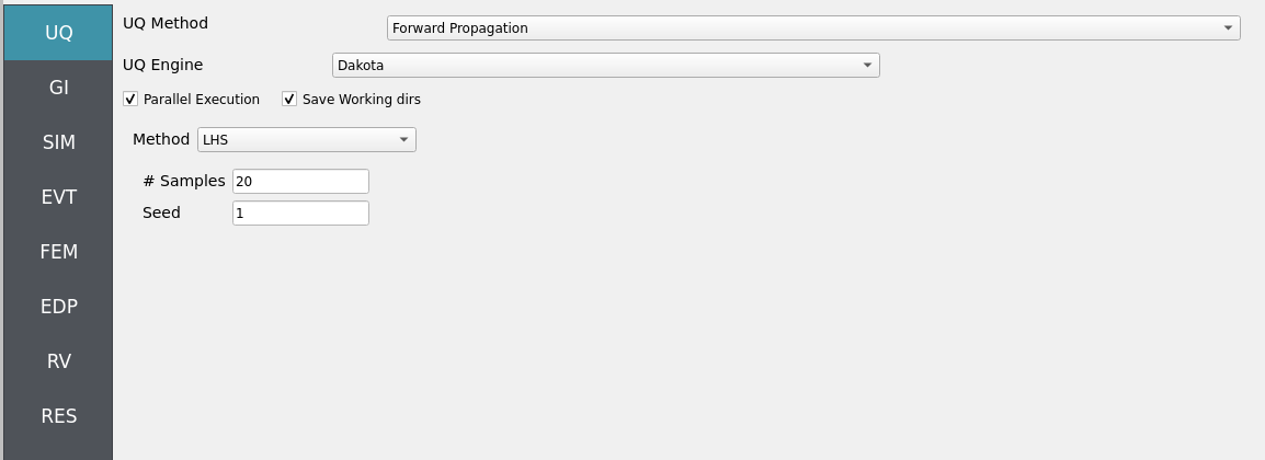
4.6.2.1. Step 1: UQ
Configure Forward sampling to explore structural/material uncertainty under a fixed hydrodynamic signal.
Engine: Dakota
Forward Propagation: Sampling method (e.g., LHS) with
samples(e.g.,20) and a reproducibleseed(e.g.,1).
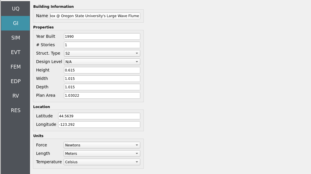
4.6.2.2. Step 2: GI
Set General Information and Units consistent with the OSU LWF experiments (length, time, density, gravity). Record project metadata.
Structure name:
Raised Structural Box @ Oregon State University's Large Wave FlumeUnits: choose a consistent set (e.g., N-m-s or kips-in-s)
Note
Keep GI, SIM, EVT, and FEM units consistent. Match MPM’s length/time scales and OpenSees integration settings (e.g., time step). Verify any force/unit conversions used during load mapping.
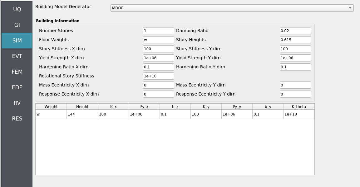
4.6.2.3. Step 3: SIM
The structural model is as follows: a single-story Multi-Degree-of-Freedom system (MDOF, see Multiple Degrees of Freedom (MDOF)) which we vertically invert to replicate the hanging, raised structural box in the OSU LWF tests.
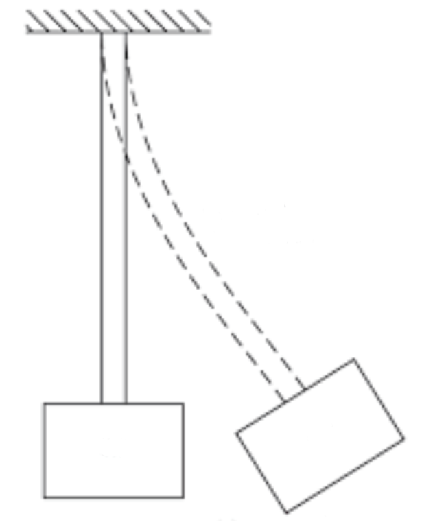
Fig. 4.6.2.3.1 Schematic of a single-story MDOF structure representing a structural box undergoing deflection from MPM derived hydrodynamic loading.
Note
The structure will be represented initially as a rigid boundary in MPM to recover local hydrodynamic forces at grid nodes for direct comparison with load-cell data. Structural dynamic response is added later by mapping these loads onto an OpenSees model defined here in the SIM panel with analysis options set in the FEM panel.
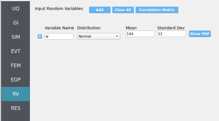
Uncertain structural properties (treated as RVs; see Step 7):
w: Weight. Mean144, stdev12
Bind parameters via setting alphabetic characters in the variable input boxes (e.g., w) so the RV panel recognizes and manages them automatically.
While not necessary to have, we show the template OpenSees model for your reference. The script generated in the backend by the MDOF module resembles the following, MDOF.tcl:
Click to expand the OpenSees input file used for this example
 1model BasicBuilder -ndm 3 -ndf 6
 2pset w 144.0
 3node 2 0 0 576 -mass $w $w  0.0  0.0  0.0  0.0
 4fix 2 0 0 1 1 1 0
 5node 1 0 0 0
 6fix 1 1 1 1 1 1 1
 7uniaxialMaterial Steel01 1 1e+06 100 0.1
 8uniaxialMaterial Steel01 2 1e+06 100 0.1
 9uniaxialMaterial Elastic 3 1e+10
10element zeroLength 1 1 2 -mat 1 2 3 -dir 1 2 6 -doRayleigh
4.6.2.4. Step 4: EVT
In this walk-through we will give a detailed step-by-step configuration of the MPM EVT module.
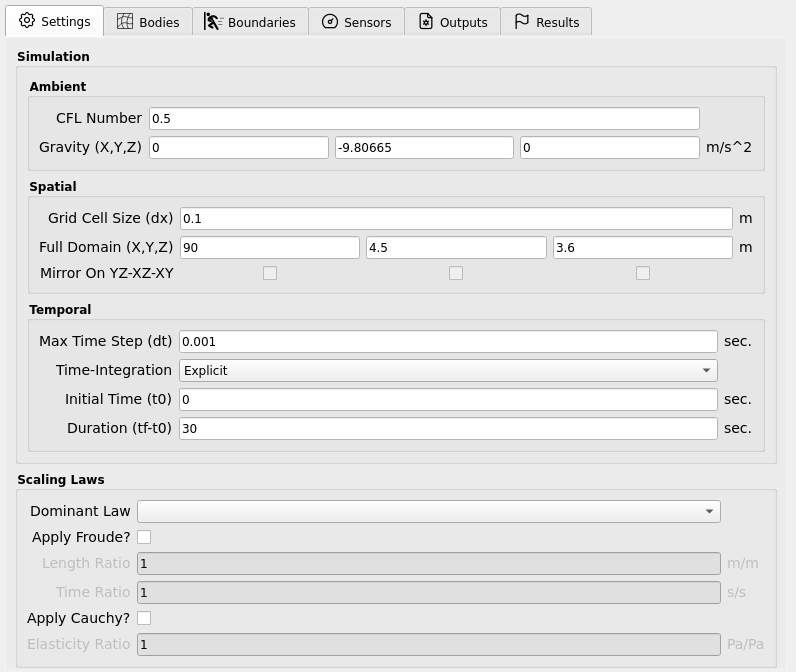
Settings
Open Settings. Here we set the simulation time, the time step, and the grid resolution, among other pre-simulation decisions.
Bodies
Geometry
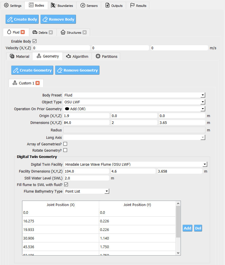
Fluid geometry
Open Bodies / Fluid / Geometry. Here we set the geometry of the flume’s fluid. Note that it is simply a rectangular prism which will be modified to be flush with the defined flume bathymetry.
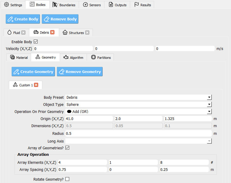
Debris geometry:
Open Bodies / Debris / Geometry. Here we set the debris properties, such as the number of debris, the size of the debris, and the spacing between the debris. Rotation is another option, though not used in this example. We’ve elected to use an 4 x 8 grid of debris (longitudinal axis parallel to long-axis of the flume).
Material
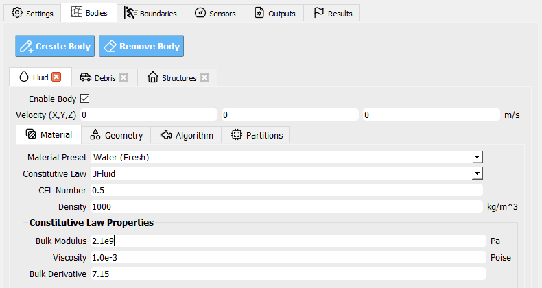
Fluid material:
Open Bodies / Fluid / Material. Here we set the material properties of the fluid. You may choose to use a realistic bulk modulus value of 2.1 GPa for the water, or you may soften it to 0.21 GPa to accelerate the simulation and reduce numerical stiffness with fairly minimal changes in our final results.
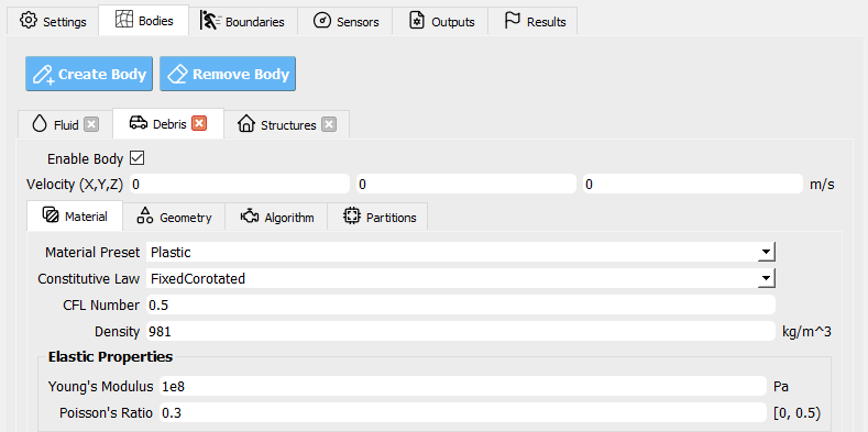
Debris material:
Moving onto the creation of an ordered debris array, we set the debris properties in the Bodies / Debris / Material tab. We will assume debris are made of HDPE plastic, as in experiments by Mascarenas 2022 [Mascarenas2022] and Shekhar et al. 2020 [Shekhar2020], and set properties accordingly.
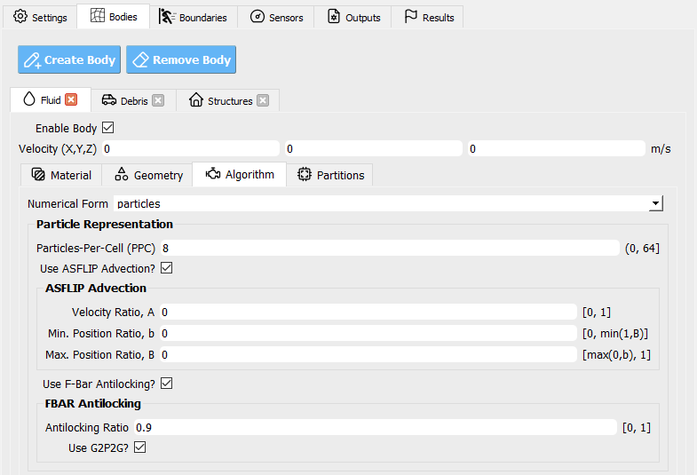
Algorithm
Open Bodies / Fluid / Algorithm. Here we set the algorithm parameters for the simulation. This is an advanced feature of the MPM module, it is best not to alter it too much. We choose to apply F-Bar antilocking to aid in the pressure field’s accuracy on the fluid. The associated toggle must be checked, and the antilocking ratio set to 0.9, loosely. For full bulk modulus water, you may need to increase this value to alleviate numerical stiffness. ASFLIP is also turned on to allow tracking of individual water particle velocities.
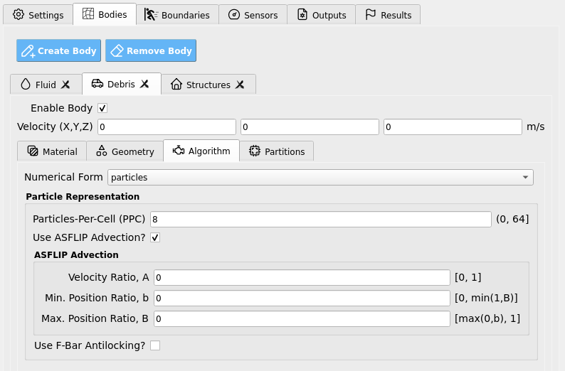
In Bodies / Debris / Algorithm we set debris for compatibility with the fluid as follows: ASFLIP is turned on and F-Bar antilocking is turned off. We keep ASFLIP tuning values at their default of zero as we do not need advanced behavior in this example.
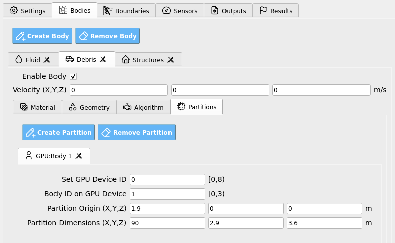
Partitions:
Open Bodies / Fluid / Partitions. This is an advanced feature of the MPM module which allows us to partition material bodies across hardware devices to optimize simulations. These may be kept as their default values, which have already been set for compatibility on the remote HPC system.
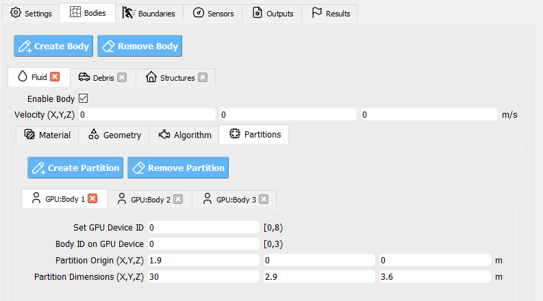
Next, Bodies / Debris / Partitions defines a partition where the debris may exist in our flume domain and defines the hardware device (i.e., GPU) that they will be simulated on. Note that it occupies the same GPU device as part of the fluid, but as a different model. Keep this as the default unless you are an advanced user.
Structure:
Finally, open Bodies / Structures. Uncheck the box that enables this body. We will not model the structure as a deformable MPM material body in this example, instead, we will approximate it as a rigid MPM boundary a few steps from now. After the MPM simulation we will map loads from the boundary to an OpenSees structure for structural analysis, see Steps 3 and 5 for configuration.
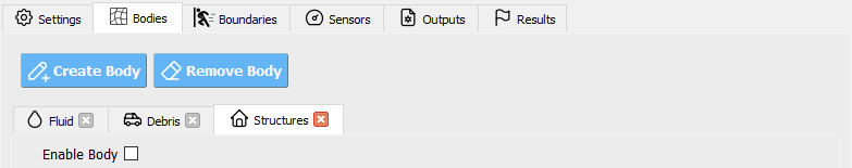
Fig. 4.6.2.4.1 HydroUQ Bodies Structures GUI
Boundaries
Wave Flume boundary:
Open Boundaries / Flume Facility. We will set the flume boundary to be a rigid body, with a fixed separable velocity condition. Bathymetry joint points should be identical to the ones used in Bodies / Fluid / Geometry.
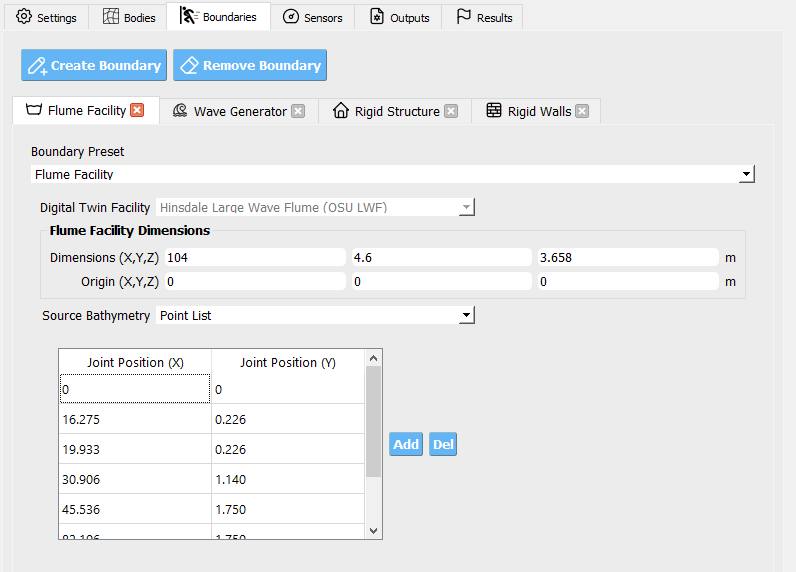
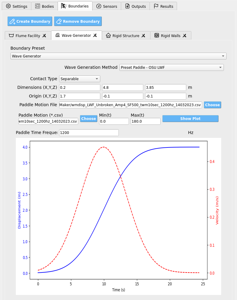
Wave Generator:
Open Boundaries / Wave Generator. Fill in the appropriate file-path for the wave generator paddle motion, wmdisp_LWF_Unbroken_Amp4_SF500_twm10sec_1200hz_14032023.csv. It is designed to produce solitary-like waves to replicate properties of a tsunami wave after it broaches the bathymetry crest.
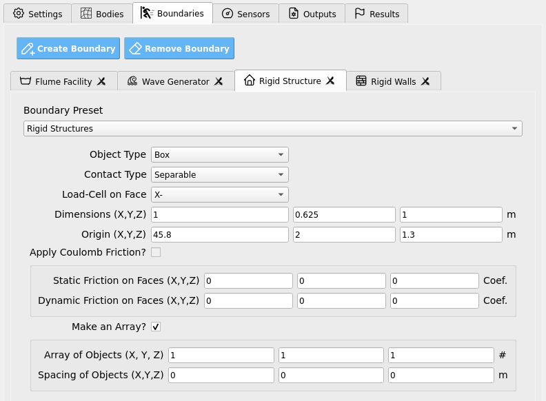
Rigid Structure:
Open Boundaries / Rigid Structure. This is where we will specify the structure as a boundary condition. By doing so, we can determine the exact loads on the rigid boundary grid-nodes, which automatically map to the model defined in the SIM and FEM tab in Steps 3 and 5 for potentially nonlinear UQ structural response analysis.
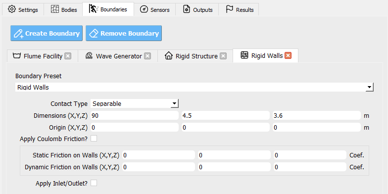
Rigid Walls:
Open Boundaries / Rigid Walls. Set to encompass the flume domain.
Sensors
Wave Gauges:
Open Sensors / Wave Gauges. Set the Use these sensor? box to True so that the simulation will output results for the instruments we set on this page.
Three wave gauges will be defined. The first is located prior to the bathymetry ramps, the second partially up the ramps, and the third near the bathymetry crest, debris, and raised structure.
Set the origins and dimensions of each wave gauge to encompass at least one grid-cell in each direction as in the table below. To match experimental conditions, we also apply a 30 Hz sampling rate to the wave gauges.
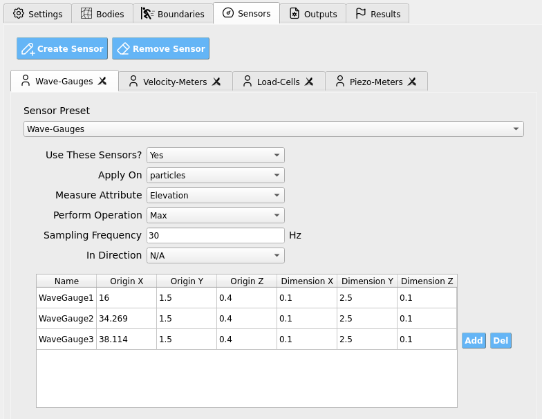
These wave gauges will read all numerical bodies (i.e. particles) within their defined regions at every sampling step and will report the highest elevation value (Position Y) of a contained body as the free-surface elevation at that gauge. The results are written into our sensor results files which we will later analyze.
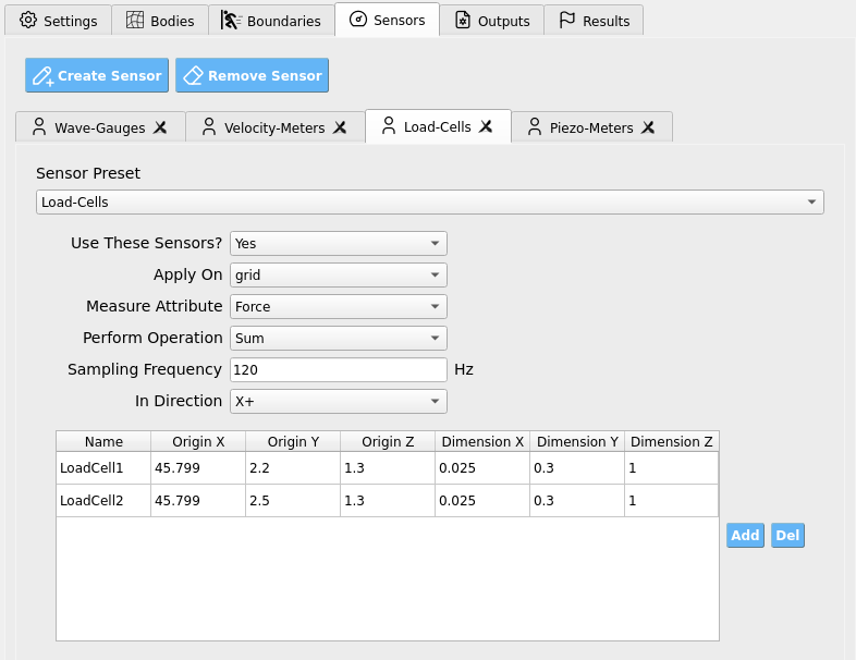
Load Cells:
Open Sensors / Load Cells. Set the Use these sensor? box to True so that the simulation will output results for the instruments we set on this page. Two load cells are defined so that we may map loads onto two nodes of our OpenSees structural model which we defined in Steps 3 and 5. Output frequency is set to 1200 Hz to match experiments and capture primary load phenomena.
Outputs
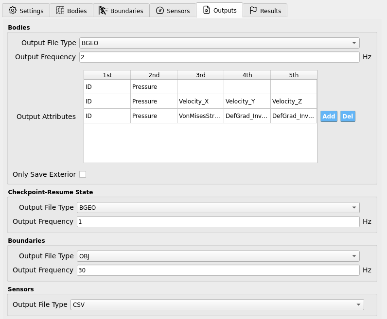
Open Outputs. Here we set the non-physical output parameters for the simulation, e.g. attributes to save per frame and file extension types. The particle bodies’ output frequency is set to 2 Hz, meaning the simulation will output results every 0.5 seconds. This is to save disk space and reduce I/O load, but it may be increased if you wish to make animations (e.g., 10 - 30 Hz). Fill the rest of the data in the figure into your GUI to ensure all your outputs match this example. You may alter output attributes if you are an advanced user familiar with ClaymoreUW attributes and wish to perform more advanced analysis.
4.6.2.5. Step 5: FEM
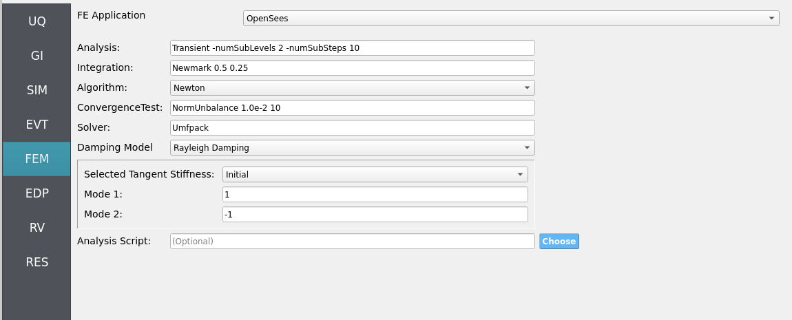
This example insofar focused on hydrodynamic forces measured on rigid structures. To perform true structural response analysis, map recovered boundary loads to an OpenSees model in SIM and configure dynamic analysis here as in other HydroUQ tutorials.
Solver: OpenSees dynamic analysis. Check:
Integration step compatible with MPM sensor output interval.
Algorithm/convergence tolerances suitable for expected nonlinearity.
Damping model as needed (e.g., Rayleigh).
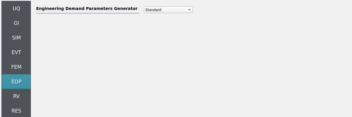
4.6.2.6. Step 6: EDP
Select Engineering Demand Parameters (EDPs) to summarize response:
Peak Floor Acceleration (PFA)
Root Mean Square Acceleration (RMSA)
Peak Floor Displacement (PFD)
Peak Interstory Drift (PID)
4.6.2.7. Step 7: RV
Define distributions for structural RV:
Structural
w: Normal (mean144, stdev12)
For future UQ, consider debris-field parameters (size, spacing, orientation, ordering), wave amplitude/period, and bathymetry tolerances as random variables.
4.6.3. Simulation
This case was executed on TACC Stampede3 using 2x NVIDIA H100 GPUs on a single node (queue: h100).
Simulated physical time: 30 s. Wall time: 2 h (allow ample Max Run Time in job settings).
Important
Provide generous Max Run Time, on the order of 90 to 120 minutes, to complete the run and post-processing before scheduler limits are reached.
Warning
Keep sensor regions, counts, sampling rates, and output frequencies reasonable—excess I/O can dominate runtime.
Outputs
Sensor CSVs (gauges, debris CoM, loads) at your chosen rates.
Particle/field snapshots (e.g., BGEO/VTK) for visualization/diagnostics.
4.6.4. Analysis
Accessing Results and Simulation Files
When the simulation job has been completed, the results and simulation files will be available on the remote system for retrieval or remote post-processing.
Retrieving the results.zip, templatedir.zip, workdir.tar.gz, and MPM folders will allow you to analyze all of the simulation output (e.g., hydrodynamic, structural, uncertainty quantification).
results.zip: Contains primary uncertainty quantification output and MPM sensor files. This will be the primary place for analysis.templatedir.zip: Contains template and workflow files for the job. This is an important resource for debugging your workflows.workdir.tar.gz: Contains the working directories in which each unique simulation was ran. This is where structural response uncertainty is expanded on typically.MPM: Contains all the MPM simulation files. Includes the raw particle output frames which can be used to create animations or to perform more advanced post-processing.
The most straightforward way to retrieve the most important files, results.zip and templatedir.zip, is by clicking the GET From DesignSafe button in HydroUQ.

Fig. 4.6.4.1 HydroUQ GET From DesignSafe button, which opens up a jobs table of all your remote simulations.
Then, right-click on your job (if it is finished) and select Retrieve Data. This will download results.zip and templatedir.zip.
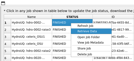
Fig. 4.6.4.2 Locating the Retrieve Data button in the HydroUQ remote jobs table.
HydroUQ will then automatically unzip them into results and templatedir, which will be located in {your_path}/HydroUQ/RemoteWorkDir/tmp.SimCenter. On most systems, this will be ~/Documents/HydroUQ/RemoteWorkDir/tmp.SimCenter, but you can check by clicking on Files / Preferences on the upper-left corner of HydroUQ.
To retrieve workdir.tar.gz and MPM, there are two approaches:
You can right-click on your job within HydroUQ and select
Open Job Folderto be taken directly to the Design Safe web-page displaying all remote files.
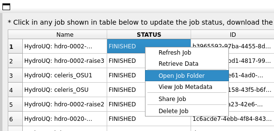
Fig. 4.6.4.3 Locating the Open Job Folder button in the HydroUQ remote jobs table.
You can manually navigate to the designsafe-ci.org website. For the latter, login and go to
Upper-right Drop-down/Job Status.

Fig. 4.6.4.4 Locating the job files on DesignSafe
Check if the job has finished in the central vertical drawer by refreshing the page. If it has, click View Details.
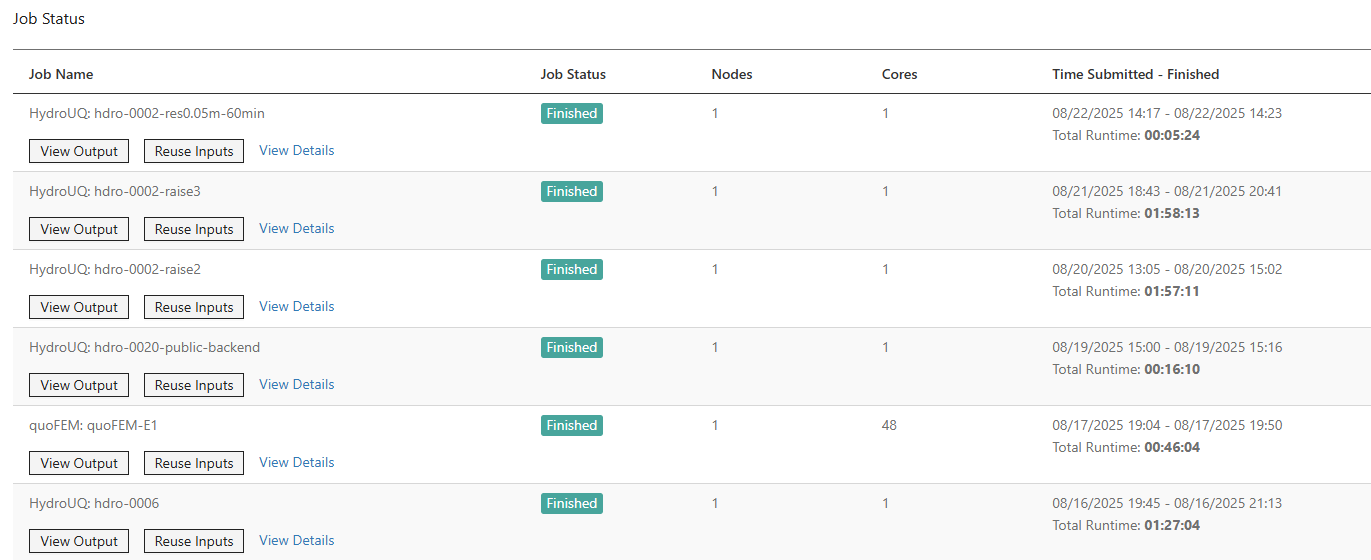
Fig. 4.6.4.5 Job status is finished on DesignSafe
Once the job is finished, the output files should be available in the directory which the analysis results were sent to
Find the files by clicking View Output.
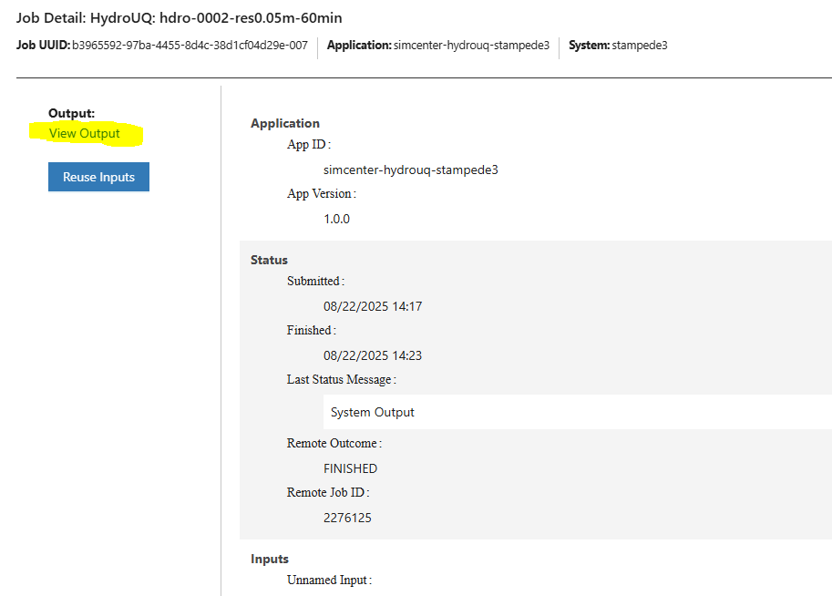
Fig. 4.6.4.6 Viewing the job files on DesignSafe
After navigating to your job folder by one of two ways, it is time to move files for processing. Move important files to somewhere in My Data/ for easier processing. Use the extractor tool available on DesignSafe to unzip the results.zip, workdir.tar.gz, and templatedir.zip folders natively on DesignSafe.
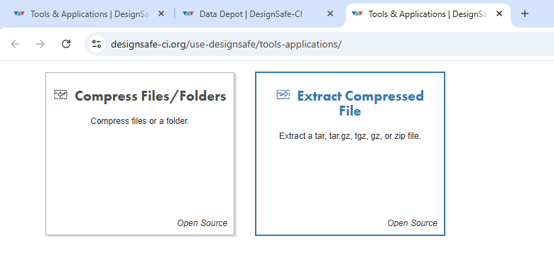
Fig. 4.6.4.7 Extracting the results.zip folder on DesignSafe
Alternatively, you may directly download the zipped folders to your PC, which will require you to use the DesignSafe zip tool on the MPM folder prior.
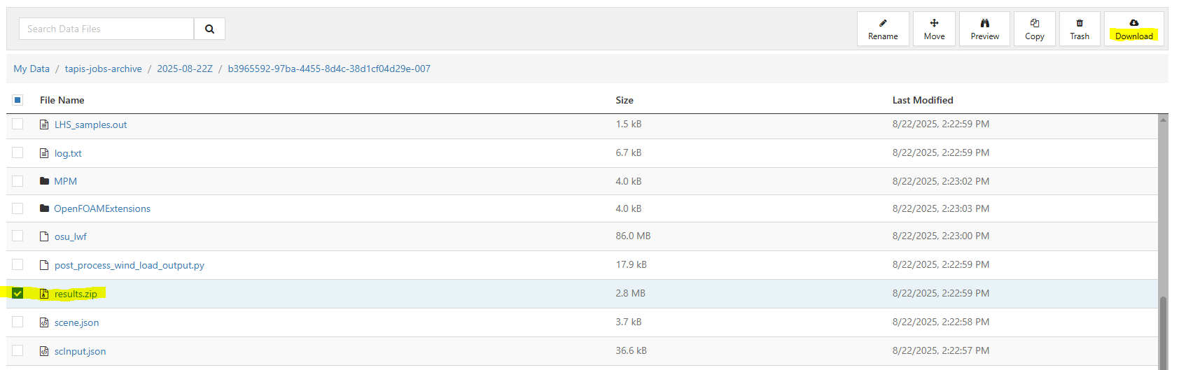
Fig. 4.6.4.8 Download button on DesignSafe shown in red
Locate the downloaded zip folders and extract them somewhere convenient. The HydroUQ local or remote work directory on your computer is a good option.
Warning
Files in the HydroUQ local and remote working directories may be erased if another simulation is set up in HydroUQ, so keep a backup if you wish to maintain the files.
Particle geometry files often have a BGEO extension and are located in the MPM folder. Open with Side FX Houdini Apprentice (free to use) to look at MPM results in high-detail, or use the PartIO library.
HydroUQ’s sensor/probe/instrument output is available in {your_path}/HydroUQ/RemoteWorkDir/tmp.SimCenter/results/ as CSV files. You may process these files as you wish, most opt to use custom Python scripts or Excel due to their simplicity.
Note
For convenience, HydroUQ also includes basic plotting of all sensors files in the EVT / Results tab. Click Post-Process Sensors, configure the drop-down boxes for the sensor you wish to view, and then click Plot.
Plotting the wave gauges shows the development of a solitary-like wave as it propagates over the bathymetry.
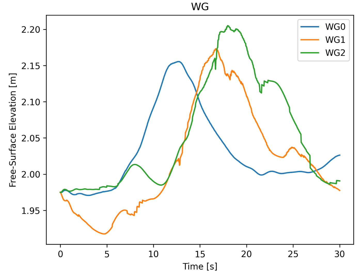
Fig. 4.6.4.9 Simulated free-surface elevations at three wave gauges in MPM.
Load-cell data shows an initially high peak force from debris impact, followed by some damming forces and eventually just hydrodynamic drag. A first peak max load of approximately 1900 Newtons is seen. We will compare this to stochastic experiments later and see that it is a reasonable estimate.
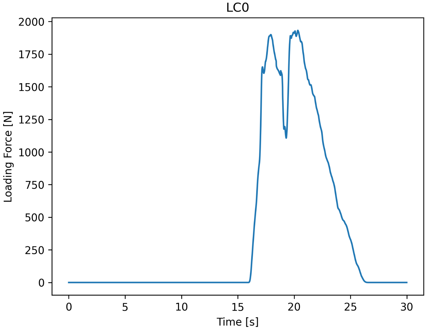
Fig. 4.6.4.10 Simulated load-cell forces in MPM. These are later mapped onto an OpenSees structure for dynamic response analysis.
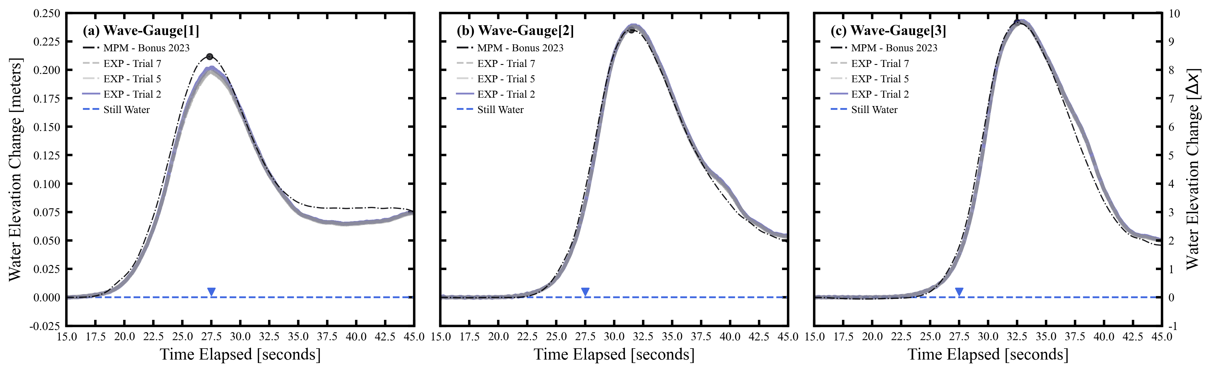
While this example concerned a quick-to-run simulation with around a million particles at a grid-resolution of 0.1 meters, higher resolution cases with 100 million particles and 0.025 meter cells are possible on remote HPC systems, including Stampede3 and Lonestar6. Below we show simulation results at these specifications from [Bonus2023Dissertation] compared against experiments to demonstrate the benefit of increased resolution. These simulations took 24 hours to complete. We emphasize these high-resolution results are possible in HydroUQ for advanced users, but may be more readily achieved by using ClaymoreUW MPM natively as advanced memory management features not exposed in the HydroUQ GUI can become important.
Wave-gauge validation (WG1-WG3) vs Mascarenas 2022 “unbroken” solitary wave:
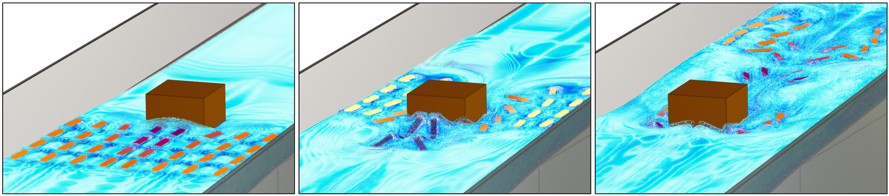
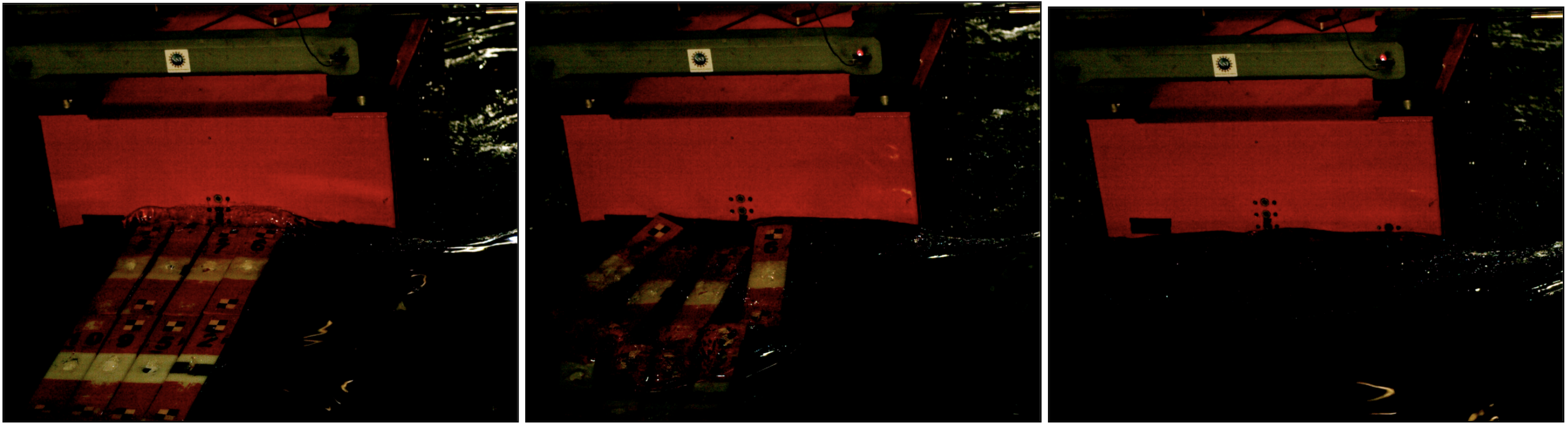
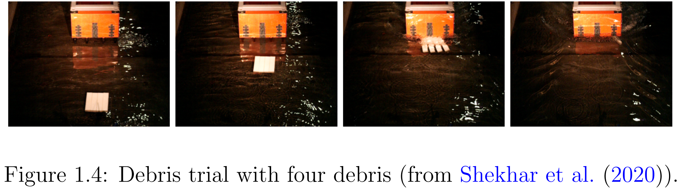
Qualitative comparison of debris impact, stalling, and deflection in high resolution simulations ([Bonus2023Dissertation]) vs experimental observations from Mascarenas (2022). We recommend you take the time to download geometry files from the remote MPM folder and visualize this scene yourself in SideFX Houdini Apprentice to view the affect of simulation resolution on these phenomena.
Alternate configuration (Shekhar et al. 2020): debris placed 0.5 m upstream relative to the box and water level 0.10–0.15 m lower than the 2.0-m datum used in our simulation and Mascarenas (2022) tests. Readers may try to replicate this case if motivated.
Ensemble comparison (optional). Box-and-whisker charts across multiple ordered debris-array cases show simulated first-peak impact forces largely within experimental IQRs and envelopes. As our simulation in this example corresponds to the 16-L-2.0x0.4 case, our first peak impact load of 1900 Newtons falls at the lower-end of the interquartile range of experiments, suggesting our results are reasonable.

Note
This HydroUQ example runs the MPM configuration natively. Experimental results can be imported (optional) for side-by-side plots in the Analysis section for a comparative study, as in Bonus (2023). Acquire said data from: PRJ-2906.
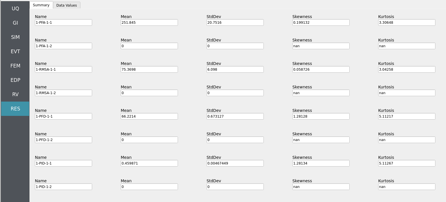
Structural Analysis
Returning to our primary HydroUQ workflow, which concerns uncertainty in structural response, we may now view the final results in the RES tab. Clicking Summary on the top-bar, a statistical summary of results is shown below:
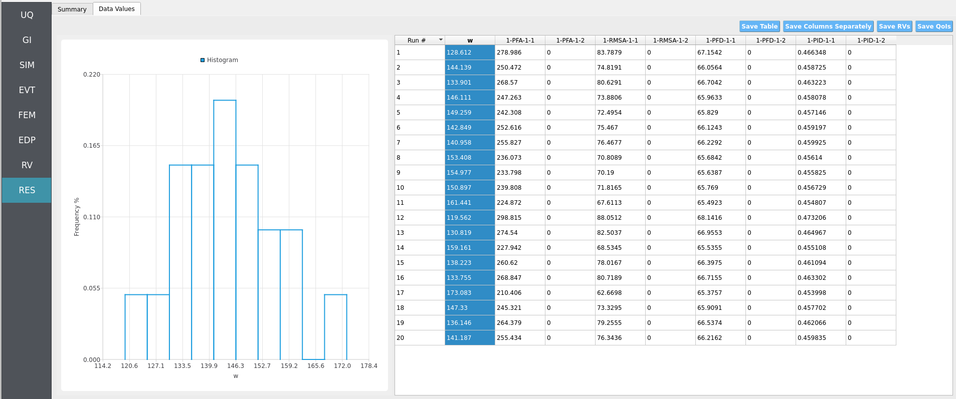
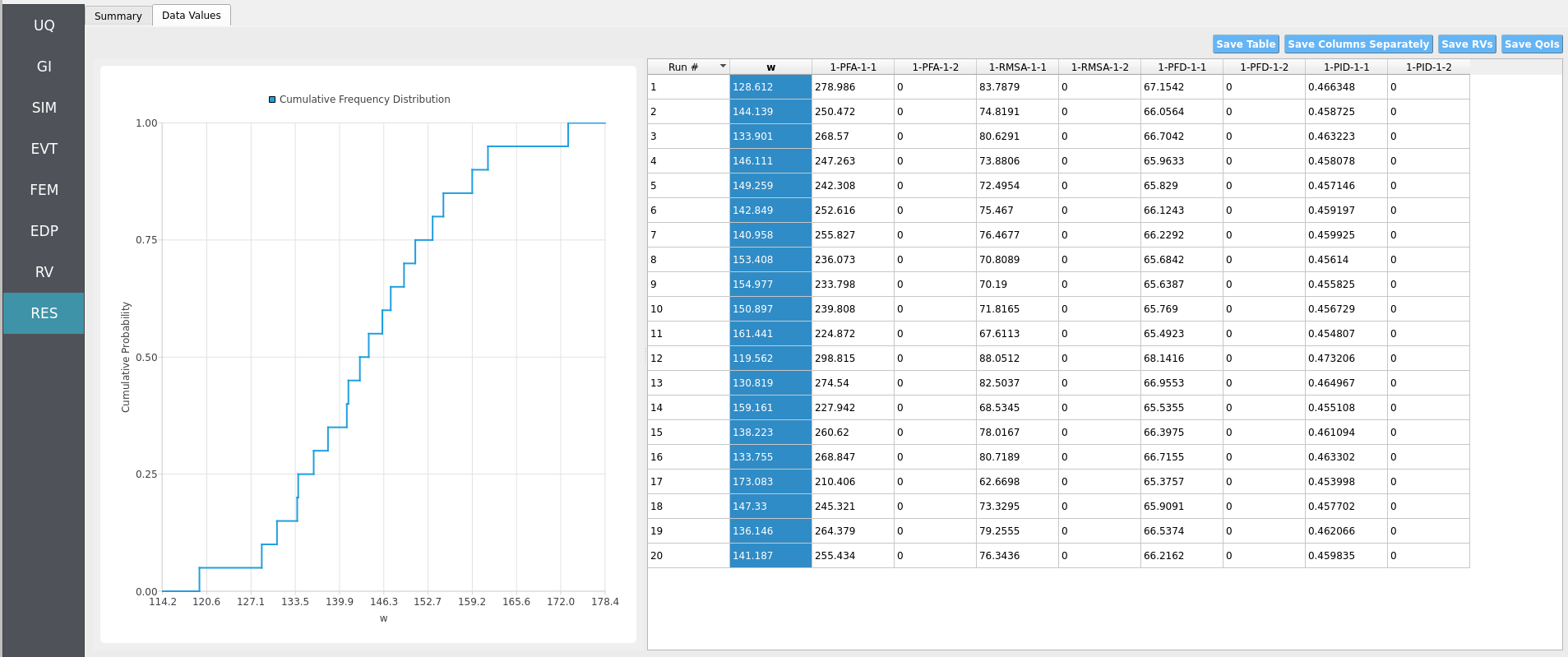
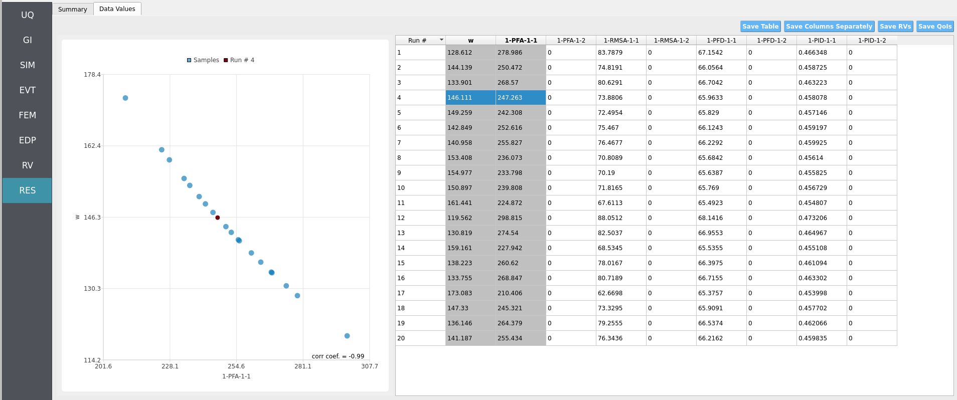
Clicking Data Values on the top-bar shows detailed histograms, cumulative distribution functions, and scatter plots relating the dependent and independent variables:
Note
In the Data Values tab, left- and right-click column headers to change plot axes; selecting a single column with both clicks displays frequency and CDF plots.
Note
Use consistent Froude similitude scaling when comparing numerical simulations, experiments, and full-scale scenarios. For cross-method comparisons, adopt identical debris footprints, friction models, probe placement, and other pertinent parameters to reduce bias.
For more advanced analysis, export results as a CSV file by clicking Save Table on the upper-right of the application window. This will save the independent and dependent variable data. I.e., the Random Variables you defined and the Engineering Demand Parameters determined from the structural response per each simulation.
To save your simulation configuration with results included, click File / Save As and specify a location for the HydroUQ JSON input file to be recorded to. You may then reload the file at a later time by clicking File / Open. You may also send it to others by email or place it in an online repository for research reproducibility. This example’s input file is viewable at Reproducibility.
To directly share your simulation job and results in HydroUQ with other DesignSafe users, click GET from DesignSafe. Then, navigate to the row with your job and right-click it. Select Share Job. You may then enter the DesignSafe username or usernames (comma-separated) to share with.
Important
Sharing a job requires that the job was initially ran with an Archive System ID (listed in the GET from DesignSafe table’s columns) that is not designsafe.storage.default. Any other Archive System ID allows for sharing with DesignSafe members on the associated project. See Jobs for more details.
4.6.5. Conclusions
HydroUQ’s OSU LWF digital flume + MPM reproduces key laboratory observations of debris-field impacts on a raised structure, with wave-gauge signals and streamwise load-cell forces in good agreement with experiments. Differences between Shekhar (2020) and Mascarenas (2022) configurations (debris start position and water level) are captured, indicating low bias to minor setup variations. The workflow is ready for scaling to UQ studies (e.g., debris-field ordering/spacing/size).
4.6.6. References
Winter, A. (2019). “Effects of Flow Shielding and Channeling on Tsunami-Induced Loading of Coastal Structures.” PhD thesis. University of Washington, Seattle.
Andrew O Winter, Mohammad S Alam, Krishnendu Shekhar, Michael R Motley, Marc O Eberhard, Andre R Barbosa, Pedro Lomonaco, Pedro Arduino, Daniel T Cox (2019). “Tsunami-Like Wave Forces on an Elevated Coastal Structure: Effects of Flow Shielding and Channeling.” Journal of Waterway, Port, Coastal, and Ocean Engineering.
Shekhar, K., Mascarenas, D., and Cox, D. (2020). “Wave-Driven Debris Impact on a Raised Structure in the Large Wave Flume.” 17th International Conference on Hydroinformatics, Seoul, South Korea.
Mascarenas, Dakota. (2022). “Quantification of Wave-Driven Debris Impact on a Raised Structure in a Large Wave Flume.” Masters thesis. University of Washington, Seattle.
Mascarenas, Dakota, Motley, M., Eberhard, M. (2022). “Wave-Driven Debris Impact on a Raised Structure in the Large Wave Flume.” Journal of Waterway, Port, Coastal, and Ocean Engineering.
Bonus, Justin (2023). “Evaluation of Fluid-Driven Debris Impacts in a High-Performance Multi-GPU Material Point Method.” PhD thesis. University of Washington, Seattle.
Justin Bonus, Felix Spröer, Andrew Winter, Pedro Arduino, Clemens Krautwald, Michael Motley, Nils Goseberg (2025). “Tsunami Debris Motion and Loads in a Scaled Port Setting: Comparative Analysis of Three State-of-the-Art Methods Against Experiments.” Coastal Engineering. Volume 197. https://doi.org/10.1016/j.coastaleng.2024.104672.
Bonus, J., & Arduino, P. (2025). ClaymoreUW. Zenodo. https://doi.org/10.5281/zenodo.15128706
4.6.7. Reproducibility
Random seed(s):
1(set in UQ)App version: HydroUQ v4.2.0 (or current)
Solver: MPM (ClaymoreUW, multi-GPU)
Hardware: TACC Lonestar6 or Stampede3, 3x A100 or 4x H100 (single node,
gpu-a100orh100queue)Simulated time: 30 seconds; Wall time: 1-2 hours
Sensor sampling: wave-gauges 120 Hz; particle output 2-10 Hz
Input: The HydroUQ input file is as follows: input.json , is used:
Click to expand the HydroUQ input file used for this example
1{
2 "Applications": {
3 "EDP": {
4 "Application": "StandardEDP",
5 "ApplicationData": {
6 }
7 },
8 "Events": [
9 {
10 "Application": "MPM",
11 "ApplicationData": {
12 },
13 "EventClassification": "Hydro",
14 "defaultMaxRunTime": "1440",
15 "driverFile": "sc_driver",
16 "inputFile": "scInput.json",
17 "maxRunTime": "120",
18 "programFile": "osu_lwf",
19 "publicDirectory": "./"
20 }
21 ],
22 "Modeling": {
23 "Application": "MDOF_BuildingModel",
24 "ApplicationData": {
25 }
26 },
27 "Simulation": {
28 "Application": "OpenSees-Simulation",
29 "ApplicationData": {
30 }
31 },
32 "UQ": {
33 "Application": "Dakota-UQ",
34 "ApplicationData": {
35 }
36 }
37 },
38 "DefaultValues": {
39 "driverFile": "driver",
40 "edpFiles": [
41 "EDP.json"
42 ],
43 "filenameAIM": "AIM.json",
44 "filenameDL": "BIM.json",
45 "filenameEDP": "EDP.json",
46 "filenameEVENT": "EVENT.json",
47 "filenameSAM": "SAM.json",
48 "filenameSIM": "SIM.json",
49 "rvFiles": [
50 "AIM.json",
51 "SAM.json",
52 "EVENT.json",
53 "SIM.json"
54 ],
55 "workflowInput": "scInput.json",
56 "workflowOutput": "EDP.json"
57 },
58 "EDP": {
59 "type": "StandardEDP"
60 },
61 "Events": [
62 {
63 "Application": "MPM",
64 "EventClassification": "Hydro",
65 "example": "OSU LWF",
66 "bodies": [
67 {
68 "algorithm": {
69 "ASFLIP_alpha": 0,
70 "ASFLIP_beta_max": 0,
71 "ASFLIP_beta_min": 0,
72 "FBAR_fused_kernel": true,
73 "FBAR_psi": 0.9,
74 "ppc": 8,
75 "type": "particles",
76 "use_ASFLIP": false,
77 "use_FBAR": true
78 },
79 "geometry": [
80 {
81 "apply_array": false,
82 "apply_rotation": false,
83 "body_preset": "Fluid",
84 "facility": "Hinsdale Large Wave Flume (OSU LWF)",
85 "facility_dimensions": [
86 104,
87 4.6,
88 3.6
89 ],
90 "fill_flume_upto_SWL": true,
91 "object": "OSU LWF",
92 "offset": [
93 1.9,
94 0,
95 0
96 ],
97 "operation": "add",
98 "span": [
99 84,
100 2,
101 3.6
102 ],
103 "standing_water_level": 2,
104 "track_particle_id": [
105 0
106 ],
107 "use_custom_bathymetry": false
108 }
109 ],
110 "gpu": 0,
111 "material": {
112 "CFL": 0.5,
113 "bulk_modulus": 210000000,
114 "constitutive": "JFluid",
115 "gamma": 7.15,
116 "material_preset": "Water (Fresh)",
117 "rho": 1000,
118 "viscosity": 0.001
119 },
120 "model": 0,
121 "name": "fluid",
122 "output_attribs": [
123 "ID",
124 "Pressure"
125 ],
126 "partition": [
127 {
128 "gpu": 0,
129 "model": 0,
130 "partition_end": [
131 31.9,
132 2.9,
133 3.6
134 ],
135 "partition_start": [
136 1.9,
137 0,
138 0
139 ]
140 },
141 {
142 "gpu": 1,
143 "model": 0,
144 "partition_end": [
145 91.9,
146 2.9,
147 3.6
148 ],
149 "partition_start": [
150 31.9,
151 0,
152 0
153 ]
154 },
155 {
156 "gpu": 2,
157 "model": 0,
158 "partition_end": [
159 121.9,
160 2.9,
161 3.6
162 ],
163 "partition_start": [
164 91.9,
165 0,
166 0
167 ]
168 }
169 ],
170 "partition_end": [
171 31.9,
172 2.9,
173 3.6
174 ],
175 "partition_start": [
176 1.9,
177 0,
178 0
179 ],
180 "target_attribs": [
181 "Position_Y"
182 ],
183 "track_attribs": [
184 "Position_X",
185 "Position_Z",
186 "Pressure"
187 ],
188 "track_particle_id": [
189 0
190 ],
191 "type": "particles",
192 "velocity": [
193 0,
194 0,
195 0
196 ]
197 },
198 {
199 "algorithm": {
200 "ASFLIP_alpha": 0,
201 "ASFLIP_beta_max": 0,
202 "ASFLIP_beta_min": 0,
203 "FBAR_fused_kernel": true,
204 "FBAR_psi": 0,
205 "ppc": 8,
206 "type": "particles",
207 "use_ASFLIP": true,
208 "use_FBAR": false
209 },
210 "geometry": [
211 {
212 "apply_array": true,
213 "apply_rotation": true,
214 "array": [
215 4,
216 1,
217 4
218 ],
219 "body_preset": "Debris",
220 "facility": "Hinsdale Large Wave Flume (OSU LWF)",
221 "facility_dimensions": [
222 84,
223 4.5,
224 3.6
225 ],
226 "fulcrum": [
227 0,
228 0,
229 0
230 ],
231 "object": "Box",
232 "offset": [
233 40.3,
234 2,
235 0.3
236 ],
237 "operation": "add",
238 "rotate": [
239 0,
240 0,
241 0
242 ],
243 "spacing": [
244 1,
245 1,
246 1
247 ],
248 "span": [
249 0.5,
250 0.05,
251 0.1
252 ],
253 "track_particle_id": [
254 0
255 ]
256 }
257 ],
258 "gpu": 0,
259 "material": {
260 "CFL": 0.5,
261 "constitutive": "FixedCorotated",
262 "material_preset": "Plastic",
263 "poisson_ratio": 0.3,
264 "rho": 981,
265 "youngs_modulus": 100000000
266 },
267 "model": 1,
268 "name": "debris",
269 "output_attribs": [
270 "ID",
271 "Pressure",
272 "Velocity_X",
273 "Velocity_Y",
274 "Velocity_Z"
275 ],
276 "partition": [
277 {
278 "gpu": 0,
279 "model": 1,
280 "partition_end": [
281 91.9,
282 2.9,
283 3.6
284 ],
285 "partition_start": [
286 1.9,
287 0,
288 0
289 ]
290 }
291 ],
292 "partition_end": [
293 91.9,
294 2.9,
295 3.6
296 ],
297 "partition_start": [
298 1.9,
299 0,
300 0
301 ],
302 "target_attribs": [
303 "Position_Y"
304 ],
305 "track_attribs": [
306 "Position_X",
307 "Position_Z",
308 "Pressure"
309 ],
310 "track_particle_id": [
311 0
312 ],
313 "type": "particles",
314 "velocity": [
315 0,
316 0,
317 0
318 ]
319 },
320 {
321 "algorithm": {
322 "ASFLIP_alpha": 0,
323 "ASFLIP_beta_max": 0,
324 "ASFLIP_beta_min": 0,
325 "FBAR_fused_kernel": true,
326 "FBAR_psi": 0.9,
327 "ppc": 8,
328 "type": "particles",
329 "use_ASFLIP": false,
330 "use_FBAR": true
331 },
332 "geometry": [
333 {
334 "apply_array": false,
335 "apply_rotation": false,
336 "body_preset": "Fluid",
337 "facility": "Hinsdale Large Wave Flume (OSU LWF)",
338 "facility_dimensions": [
339 104,
340 4.6,
341 3.6
342 ],
343 "fill_flume_upto_SWL": true,
344 "object": "OSU LWF",
345 "offset": [
346 1.9,
347 0,
348 0
349 ],
350 "operation": "add",
351 "span": [
352 84,
353 2,
354 3.6
355 ],
356 "standing_water_level": 2,
357 "track_particle_id": [
358 0
359 ],
360 "use_custom_bathymetry": false
361 }
362 ],
363 "gpu": 1,
364 "material": {
365 "CFL": 0.5,
366 "bulk_modulus": 210000000,
367 "constitutive": "JFluid",
368 "gamma": 7.15,
369 "material_preset": "Water (Fresh)",
370 "rho": 1000,
371 "viscosity": 0.001
372 },
373 "model": 0,
374 "name": "fluid",
375 "output_attribs": [
376 "ID",
377 "Pressure"
378 ],
379 "partition": [
380 {
381 "gpu": 0,
382 "model": 0,
383 "partition_end": [
384 31.9,
385 2.9,
386 3.6
387 ],
388 "partition_start": [
389 1.9,
390 0,
391 0
392 ]
393 },
394 {
395 "gpu": 1,
396 "model": 0,
397 "partition_end": [
398 91.9,
399 2.9,
400 3.6
401 ],
402 "partition_start": [
403 31.9,
404 0,
405 0
406 ]
407 },
408 {
409 "gpu": 2,
410 "model": 0,
411 "partition_end": [
412 121.9,
413 2.9,
414 3.6
415 ],
416 "partition_start": [
417 91.9,
418 0,
419 0
420 ]
421 }
422 ],
423 "partition_end": [
424 91.9,
425 2.9,
426 3.6
427 ],
428 "partition_start": [
429 31.9,
430 0,
431 0
432 ],
433 "target_attribs": [
434 "Position_Y"
435 ],
436 "track_attribs": [
437 "Position_X",
438 "Position_Z",
439 "Pressure"
440 ],
441 "track_particle_id": [
442 0
443 ],
444 "type": "particles",
445 "velocity": [
446 0,
447 0,
448 0
449 ]
450 },
451 {
452 "algorithm": {
453 "ASFLIP_alpha": 0,
454 "ASFLIP_beta_max": 0,
455 "ASFLIP_beta_min": 0,
456 "FBAR_fused_kernel": true,
457 "FBAR_psi": 0.9,
458 "ppc": 8,
459 "type": "particles",
460 "use_ASFLIP": false,
461 "use_FBAR": true
462 },
463 "geometry": [
464 {
465 "apply_array": false,
466 "apply_rotation": false,
467 "body_preset": "Fluid",
468 "facility": "Hinsdale Large Wave Flume (OSU LWF)",
469 "facility_dimensions": [
470 104,
471 4.6,
472 3.6
473 ],
474 "fill_flume_upto_SWL": true,
475 "object": "OSU LWF",
476 "offset": [
477 1.9,
478 0,
479 0
480 ],
481 "operation": "add",
482 "span": [
483 84,
484 2,
485 3.6
486 ],
487 "standing_water_level": 2,
488 "track_particle_id": [
489 0
490 ],
491 "use_custom_bathymetry": false
492 }
493 ],
494 "gpu": 2,
495 "material": {
496 "CFL": 0.5,
497 "bulk_modulus": 210000000,
498 "constitutive": "JFluid",
499 "gamma": 7.15,
500 "material_preset": "Water (Fresh)",
501 "rho": 1000,
502 "viscosity": 0.001
503 },
504 "model": 0,
505 "name": "fluid",
506 "output_attribs": [
507 "ID",
508 "Pressure"
509 ],
510 "partition": [
511 {
512 "gpu": 0,
513 "model": 0,
514 "partition_end": [
515 31.9,
516 2.9,
517 3.6
518 ],
519 "partition_start": [
520 1.9,
521 0,
522 0
523 ]
524 },
525 {
526 "gpu": 1,
527 "model": 0,
528 "partition_end": [
529 91.9,
530 2.9,
531 3.6
532 ],
533 "partition_start": [
534 31.9,
535 0,
536 0
537 ]
538 },
539 {
540 "gpu": 2,
541 "model": 0,
542 "partition_end": [
543 121.9,
544 2.9,
545 3.6
546 ],
547 "partition_start": [
548 91.9,
549 0,
550 0
551 ]
552 }
553 ],
554 "partition_end": [
555 121.9,
556 2.9,
557 3.6
558 ],
559 "partition_start": [
560 91.9,
561 0,
562 0
563 ],
564 "target_attribs": [
565 "Position_Y"
566 ],
567 "track_attribs": [
568 "Position_X",
569 "Position_Z",
570 "Pressure"
571 ],
572 "track_particle_id": [
573 0
574 ],
575 "type": "particles",
576 "velocity": [
577 0,
578 0,
579 0
580 ]
581 }
582 ],
583 "boundaries": [
584 {
585 "contact": "Separable",
586 "domain_end": [
587 90,
588 4.6,
589 3.6
590 ],
591 "domain_start": [
592 0,
593 0,
594 0
595 ],
596 "friction_dynamic": 0,
597 "friction_static": 0,
598 "object": "OSU LWF",
599 "use_custom_bathymetry": false
600 },
601 {
602 "contact": "Separable",
603 "domain_end": [
604 1.9,
605 4.7,
606 3.75
607 ],
608 "domain_start": [
609 1.7,
610 -0.1,
611 -0.1
612 ],
613 "file": "./Examples/WaveMaker/wmdisp_LWF_Unbroken_Amp4_SF500_twm10sec_1200hz_14032023.csv",
614 "friction_dynamic": 0,
615 "friction_static": 0,
616 "object": "OSU Paddle",
617 "output_frequency": 1200
618 },
619 {
620 "array": [
621 1,
622 1,
623 1
624 ],
625 "contact": "Separable",
626 "domain_end": [
627 46.8,
628 2.825,
629 2.3
630 ],
631 "domain_start": [
632 45.8,
633 2.2,
634 1.3
635 ],
636 "friction_dynamic": 0,
637 "friction_static": 0,
638 "object": "Box",
639 "spacing": [
640 0,
641 0,
642 0
643 ]
644 },
645 {
646 "contact": "Separable",
647 "domain_end": [
648 90,
649 4.5,
650 3.6
651 ],
652 "domain_start": [
653 0,
654 0,
655 0
656 ],
657 "friction_dynamic": 0,
658 "friction_static": 0,
659 "object": "Walls"
660 }
661 ],
662 "computer": {
663 "hpc": "TACC - UT Austin - Lonestar6",
664 "hpc_card_architecture": "Ampere",
665 "hpc_card_brand": "NVIDIA",
666 "hpc_card_compute_capability": 80,
667 "hpc_card_global_memory": 40,
668 "hpc_card_name": "A100",
669 "hpc_queue": "gpu-a100",
670 "models_per_gpu": 3,
671 "num_gpus": 3
672 },
673 "grid-sensors": [
674 {
675 "attribute": "Force",
676 "direction": "X+",
677 "domain_end": [
678 45.824,
679 2.5,
680 2.3
681 ],
682 "domain_start": [
683 45.799,
684 2.2,
685 1.3
686 ],
687 "name": "LoadCell1",
688 "operation": "Sum",
689 "output_frequency": 120,
690 "preset": "Load-Cells",
691 "toggle": true,
692 "type": "grid"
693 },
694 {
695 "attribute": "Force",
696 "direction": "X+",
697 "domain_end": [
698 45.824,
699 2.8,
700 2.3
701 ],
702 "domain_start": [
703 45.799,
704 2.5,
705 1.3
706 ],
707 "name": "LoadCell2",
708 "operation": "Sum",
709 "output_frequency": 120,
710 "preset": "Load-Cells",
711 "toggle": true,
712 "type": "grid"
713 }
714 ],
715 "outputs": {
716 "bodies_output_freq": 2,
717 "bodies_save_suffix": "BGEO",
718 "boundaries_output_freq": 30,
719 "boundaries_save_suffix": "OBJ",
720 "checkpoints_output_freq": 1,
721 "checkpoints_save_suffix": "BGEO",
722 "energies_output_freq": 30,
723 "energies_save_suffix": "CSV",
724 "output_attribs": [
725 [
726 "ID",
727 "Pressure"
728 ],
729 [
730 "ID",
731 "Pressure",
732 "Velocity_X",
733 "Velocity_Y",
734 "Velocity_Z"
735 ],
736 [
737 "ID",
738 "Pressure",
739 "VonMisesStress",
740 "DefGrad_Invariant2",
741 "DefGrad_Invariant3"
742 ]
743 ],
744 "particles_output_exterior_only": false,
745 "sensors_save_suffix": "CSV",
746 "useKineticEnergy": false,
747 "usePotentialEnergy": false,
748 "useStrainEnergy": false
749 },
750 "particle-sensors": [
751 {
752 "attribute": "Elevation",
753 "direction": "N/A",
754 "domain_end": [
755 16.1,
756 4,
757 0.5
758 ],
759 "domain_start": [
760 16,
761 1.5,
762 0.4
763 ],
764 "name": "WaveGauge1",
765 "operation": "Max",
766 "output_frequency": 30,
767 "preset": "Wave-Gauges",
768 "toggle": true,
769 "type": "particles"
770 },
771 {
772 "attribute": "Elevation",
773 "direction": "N/A",
774 "domain_end": [
775 34.369,
776 4,
777 0.5
778 ],
779 "domain_start": [
780 34.269,
781 1.5,
782 0.4
783 ],
784 "name": "WaveGauge2",
785 "operation": "Max",
786 "output_frequency": 30,
787 "preset": "Wave-Gauges",
788 "toggle": true,
789 "type": "particles"
790 },
791 {
792 "attribute": "Elevation",
793 "direction": "N/A",
794 "domain_end": [
795 38.214,
796 4,
797 0.5
798 ],
799 "domain_start": [
800 38.114,
801 1.5,
802 0.4
803 ],
804 "name": "WaveGauge3",
805 "operation": "Max",
806 "output_frequency": 30,
807 "preset": "Wave-Gauges",
808 "toggle": true,
809 "type": "particles"
810 }
811 ],
812 "scaling": {
813 "cauchy_bulk_ratio": 1,
814 "froude_length_ratio": 1,
815 "froude_time_ratio": 1,
816 "use_cauchy_scaling": false,
817 "use_froude_scaling": false
818 },
819 "simulation": {
820 "cauchy_bulk_ratio": 1,
821 "cfl": 0.5,
822 "default_dt": 0.001,
823 "default_dx": 0.1,
824 "domain": [
825 90,
826 4.5,
827 3.6
828 ],
829 "duration": 30.0,
830 "fps": 2,
831 "frames": 60,
832 "froude_scaling": 1,
833 "froude_time_ratio": 1,
834 "gravity": [
835 0,
836 -9.80665,
837 0
838 ],
839 "initial_time": 0,
840 "mirror_domain": [
841 false,
842 false,
843 false
844 ],
845 "particles_output_exterior_only": false,
846 "save_suffix": ".bgeo",
847 "time": 0,
848 "time_integration": "Explicit",
849 "use_cauchy_scaling": false,
850 "use_froude_scaling": false
851 },
852 "subtype": "MPM",
853 "type": "MPM"
854 }
855 ],
856 "GeneralInformation": {
857 "NumberOfStories": 1,
858 "PlanArea": 1.030225,
859 "StructureType": "S2",
860 "YearBuilt": 2016,
861 "depth": 1.015,
862 "height": 0.615,
863 "location": {
864 "latitude": 44.5638955,
865 "longitude": -123.2915415
866 },
867 "name": "Raised Structural Box @ Oregon State University's Large Wave Flume",
868 "planArea": 1.030225,
869 "stories": 1,
870 "units": {
871 "force": "N",
872 "length": "m",
873 "temperature": "C",
874 "time": "sec"
875 },
876 "width": 1.015
877 },
878 "Modeling": {
879 "Bx": 0.1,
880 "By": 0.1,
881 "Fyx": 1000000,
882 "Fyy": 1000000,
883 "Krz": 10000000000,
884 "Kx": 100,
885 "Ky": 100,
886 "ModelData": [
887 {
888 "Fyx": 1000000,
889 "Fyy": 1000000,
890 "Ktheta": 10000000000,
891 "bx": 0.1,
892 "by": 0.1,
893 "height": 144,
894 "kx": 100,
895 "ky": 100,
896 "weight": "RV.w"
897 }
898 ],
899 "dampingRatio": 0.02,
900 "height": 144,
901 "massX": 0,
902 "massY": 0,
903 "numStories": 1,
904 "randomVar": [
905 ],
906 "responseX": 0,
907 "responseY": 0,
908 "type": "MDOF_BuildingModel",
909 "weight": "RV.w"
910 },
911 "Simulation": {
912 "Application": "OpenSees-Simulation",
913 "algorithm": "Newton",
914 "analysis": "Transient -numSubLevels 2 -numSubSteps 10",
915 "convergenceTest": "NormUnbalance 1.0e-2 10",
916 "dampingModel": "Rayleigh Damping",
917 "firstMode": 1,
918 "integration": "Newmark 0.5 0.25",
919 "modalRayleighTangentRatio": 0,
920 "numModesModal": -1,
921 "rayleighTangent": "Initial",
922 "secondMode": -1,
923 "solver": "Umfpack"
924 },
925 "UQ": {
926 "parallelExecution": true,
927 "samplingMethodData": {
928 "method": "LHS",
929 "samples": 20,
930 "seed": 1
931 },
932 "saveWorkDir": true,
933 "uqType": "Forward Propagation"
934 },
935 "localAppDir": "/home/justinbonus/SimCenter/HydroUQ/build",
936 "randomVariables": [
937 {
938 "distribution": "Normal",
939 "inputType": "Parameters",
940 "mean": 144,
941 "name": "w",
942 "refCount": 1,
943 "stdDev": 12,
944 "value": "RV.w",
945 "variableClass": "Uncertain"
946 }
947 ],
948 "remoteAppDir": "/home/justinbonus/SimCenter/HydroUQ/build",
949 "resultType": "SimCenterUQResultsSampling",
950 "runType": "runningLocal",
951 "spreadsheet": {
952 "data": [
953 1,
954 128.6117515,
955 0.00388829,
956 0,
957 0.00111096,
958 0,
959 5.43192e-06,
960 0,
961 3.77217e-08,
962 0,
963 2,
964 144.1388782,
965 0.0034605,
966 0,
967 0.000956933,
968 0,
969 5.13692e-06,
970 0,
971 3.56731e-08,
972 0,
973 3,
974 133.9007901,
975 0.00370384,
976 0,
977 0.0010505,
978 0,
979 5.3265e-06,
980 0,
981 3.69896e-08,
982 0,
983 4,
984 146.111267,
985 0.00345109,
986 0,
987 0.000941658,
988 0,
989 5.10412e-06,
990 0,
991 3.54453e-08,
992 0,
993 5,
994 149.258936,
995 0.00334116,
996 0,
997 0.000917876,
998 0,
999 5.04902e-06,
1000 0,
1001 3.50627e-08,
1002 0,
1003 6,
1004 142.8493345,
1005 0.00348563,
1006 0,
1007 0.000967186,
1008 0,
1009 5.15914e-06,
1010 0,
1011 3.58273e-08,
1012 0,
1013 7,
1014 140.9583447,
1015 0.00357113,
1016 0,
1017 0.000983426,
1018 0,
1019 5.19588e-06,
1020 0,
1021 3.60825e-08,
1022 0,
1023 8,
1024 153.4083012,
1025 0.00325312,
1026 0,
1027 0.000889362,
1028 0,
1029 4.98383e-06,
1030 0,
1031 3.46099e-08,
1032 0,
1033 9,
1034 154.9769919,
1035 0.00322062,
1036 0,
1037 0.000878716,
1038 0,
1039 4.96003e-06,
1040 0,
1041 3.44446e-08,
1042 0,
1043 10,
1044 150.8972919,
1045 0.00333385,
1046 0,
1047 0.000906788,
1048 0,
1049 5.02584e-06,
1050 0,
1051 3.49017e-08,
1052 0,
1053 11,
1054 161.4405578,
1055 0.00309876,
1056 0,
1057 0.000835724,
1058 0,
1059 4.86075e-06,
1060 0,
1061 3.37552e-08,
1062 0,
1063 12,
1064 119.5622379,
1065 0.0041708,
1066 0,
1067 0.00123468,
1068 0,
1069 5.62827e-06,
1070 0,
1071 3.90852e-08,
1072 0,
1073 13,
1074 130.819271,
1075 0.00381607,
1076 0,
1077 0.00108434,
1078 0,
1079 5.38604e-06,
1080 0,
1081 3.74031e-08,
1082 0,
1083 14,
1084 159.1607791,
1085 0.00314233,
1086 0,
1087 0.000850563,
1088 0,
1089 4.89411e-06,
1090 0,
1091 3.39868e-08,
1092 0,
1093 15,
1094 138.2232173,
1095 0.00359435,
1096 0,
1097 0.0010078,
1098 0,
1099 5.24497e-06,
1100 0,
1101 3.64234e-08,
1102 0,
1103 16,
1104 133.7552642,
1105 0.00371064,
1106 0,
1107 0.00105202,
1108 0,
1109 5.32912e-06,
1110 0,
1111 3.70078e-08,
1112 0,
1113 17,
1114 173.0828112,
1115 0.0028835,
1116 0,
1117 0.000761907,
1118 0,
1119 4.6965e-06,
1120 0,
1121 3.26146e-08,
1122 0,
1123 18,
1124 147.3303473,
1125 0.00339947,
1126 0,
1127 0.000932286,
1128 0,
1129 5.08299e-06,
1130 0,
1131 3.52986e-08,
1132 0,
1133 19,
1134 136.1464234,
1135 0.00369128,
1136 0,
1137 0.00102734,
1138 0,
1139 5.28236e-06,
1140 0,
1141 3.66831e-08,
1142 0,
1143 20,
1144 141.1872175,
1145 0.00356995,
1146 0,
1147 0.000981811,
1148 0,
1149 5.19223e-06,
1150 0,
1151 3.60572e-08,
1152 0
1153 ],
1154 "headings": [
1155 "Run #",
1156 "w",
1157 "1-PFA-1-1",
1158 "1-PFA-1-2",
1159 "1-RMSA-1-1",
1160 "1-RMSA-1-2",
1161 "1-PFD-1-1",
1162 "1-PFD-1-2",
1163 "1-PID-1-1",
1164 "1-PID-1-2",
1165 ""
1166 ],
1167 "isSurrogate": false,
1168 "nrv": 1,
1169 "numCol": 10,
1170 "numRow": 20
1171 },
1172 "summary": [
1173 {
1174 "kurtosis": 3.3693713770466243,
1175 "mean": 0.0034893190000000003,
1176 "name": "1-PFA-1-1",
1177 "skewness": 0.17680159786525307,
1178 "stdDev": 0.00030042254878753685
1179 },
1180 {
1181 "kurtosis": null,
1182 "mean": 0,
1183 "name": "1-PFA-1-2",
1184 "skewness": null,
1185 "stdDev": 0
1186 },
1187 {
1188 "kurtosis": 3.8327863239899194,
1189 "mean": 0.0009685938,
1190 "name": "1-RMSA-1-1",
1191 "skewness": 0.4760907181647112,
1192 "stdDev": 0.0001077896236796962
1193 },
1194 {
1195 "kurtosis": null,
1196 "mean": 0,
1197 "name": "1-RMSA-1-2",
1198 "skewness": null,
1199 "stdDev": 0
1200 },
1201 {
1202 "kurtosis": 3.259319365291982,
1203 "mean": 5.148527000000001e-06,
1204 "name": "1-PFD-1-1",
1205 "skewness": 0.08140336872836712,
1206 "stdDev": 2.1867144176402626e-07
1207 },
1208 {
1209 "kurtosis": null,
1210 "mean": 0,
1211 "name": "1-PFD-1-2",
1212 "skewness": null,
1213 "stdDev": 0
1214 },
1215 {
1216 "kurtosis": 3.2592302575010574,
1217 "mean": 3.575367e-08,
1218 "name": "1-PID-1-1",
1219 "skewness": 0.08138380197638177,
1220 "stdDev": 1.5185621516837287e-09
1221 },
1222 {
1223 "kurtosis": null,
1224 "mean": 0,
1225 "name": "1-PID-1-2",
1226 "skewness": null,
1227 "stdDev": 0
1228 }
1229 ],
1230 "workingDir": "/home/justinbonus/Documents/HydroUQ/LocalWorkDir"
1231}