4.2. Real-Time Wave-Solver - Simple Piston Generated Wave Loading - Taichi Event

Problem files

Github

4.2.1. Overview

Forward sample an uncertain structure loaded by a physics-based wave maker piston’s generated wave in real-time. This workflow uses the high-performance Taichi Lang on your local PC to accelerate simulations using your CPU or your GPU [Hu2019]. We numerically simulate position-based fluid dynamics (PBFD) in 2D: the right boundary is a moving wall (wave-maker piston), the center is a water particle mass, and the left is a rigid wall representing the structure onto which HydroUQ maps hydrodynamic loads for an OpenSees model. This replicates the basic physics of wave-makers in real facilities, such as Oregon State University’s Large Wave Flume and Directional Wave Basin. The OpenSees structure is a 2D three degree-of-freedom portal frame with uncertain variables.

Note

Keep GI, SIM, EVT, and FEM units consistent. Match Taichi’s PBFD length/time scales and OpenSees integration settings (e.g., time step). Verify any force/unit conversions used during load mapping.

4.2.2. Set-Up

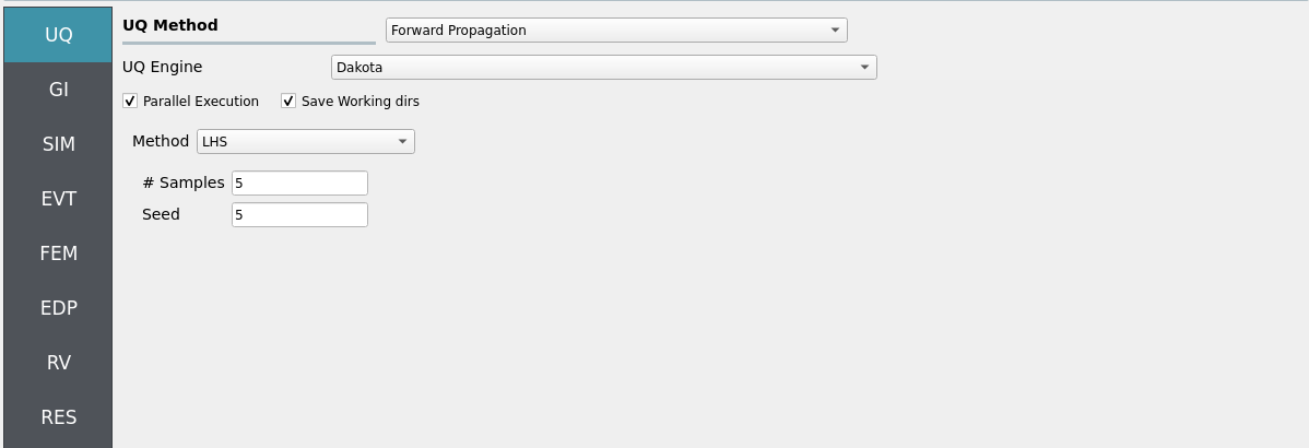
4.2.2.1. Step 1: UQ

Configure Forward sampling to explore structural/material uncertainty under a fixed piston-generated wave signal.

• Engine: Dakota

• Forward Propagation (e.g., LHS) with samples (e.g., 4) and a reproducible seed (e.g., 1).

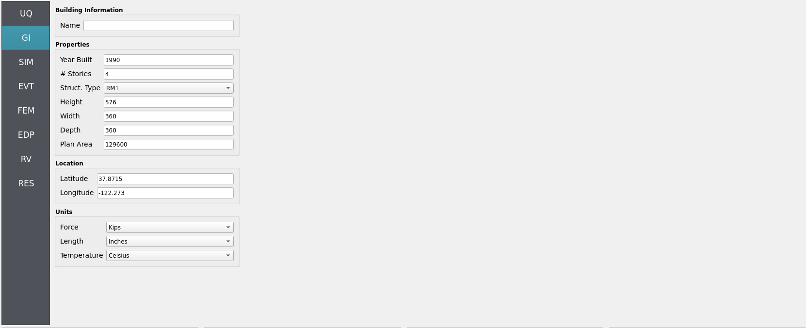
4.2.2.2. Step 2: GI

Set General Information and Units. Ensure that length/time units are consistent with the Taichi Lang script’s and OpenSees model’s parameters.

• Project name: hdro-0010

• Location/metadata: optional

• Units: choose a consistent set (e.g., N-m-s or kips-in-s)

4.2.2.3. Step 3: SIM

The structural model is as follows: a 2D, 3-DOF OpenSees portal frame in OpenSees, OpenSees.

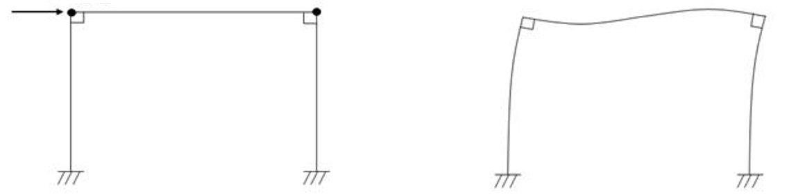
Fig. 4.2.2.3.1 2D 3-DOF portal frame under stochastic wave loading (JONSWAP)

For the OpenSees generator the following model script, Frame.tcl , is used:

Click to expand the OpenSees input file used for this example

# Create ModelBuilder (with two-dimensions and 3 DOF/node)

model basic -ndm 2 -ndf 3

set width    360
set height   144

node  1       0.0     0.0 
node  2    $width     0.0 
node  3       0.0 $height
node  4    $width $height

fix   1     1    1    1
fix   2     1    1    1

# Concrete ( Youngs Modulus, Yield Strength, and Compressive Strength)
pset fc 6.0
pset fy 60.0
pset E 30000.0
uniaxialMaterial Concrete01  1  -$fc  -0.004   -5.0     -0.014
uniaxialMaterial Concrete01  2  -5.0   -0.002   0.0     -0.006

# STEEL
uniaxialMaterial Steel01  3  $fy $E 0.01

set colWidth 15
set colDepth 24 
set cover  1.5
set As    0.60;     # area of no. 7 bars
set y1 [expr $colDepth/2.0]
set z1 [expr $colWidth/2.0]

section Fiber 1 {

    # Create the concrete core fibers
    patch rect 1 10 1 [expr $cover-$y1] [expr $cover-$z1] [expr $y1-$cover] [expr $z1-$cover]

    # Create the concrete cover fibers (top, bottom, left, right)
    patch rect 2 10 1  [expr -$y1] [expr $z1-$cover] $y1 $z1
    patch rect 2 10 1  [expr -$y1] [expr -$z1] $y1 [expr $cover-$z1]
    patch rect 2  2 1  [expr -$y1] [expr $cover-$z1] [expr $cover-$y1] [expr $z1-$cover]
    patch rect 2  2 1  [expr $y1-$cover] [expr $cover-$z1] $y1 [expr $z1-$cover]

    # Create the reinforcing fibers (left, middle, right)
    layer straight 3 3 $As [expr $y1-$cover] [expr $z1-$cover] [expr $y1-$cover] [expr $cover-$z1]
    layer straight 3 2 $As 0.0 [expr $z1-$cover] 0.0 [expr $cover-$z1]
    layer straight 3 3 $As [expr $cover-$y1] [expr $z1-$cover] [expr $cover-$y1] [expr $cover-$z1]

}    


# Define column elements
# ----------------------

# Geometry of column elements
#                tag 

geomTransf Corotational 1  

# Number of integration points along length of element
set np 5

# Create the coulumns using Beam-column elements
#               e            tag ndI ndJ nsecs secID transfTag
set eleType dispBeamColumn
element $eleType  1   1   3   $np    1       1 
element $eleType  2   2   4   $np    1       1 

# Define beam elment
# -----------------------------

# Geometry of column elements
#                tag 
geomTransf Linear 2  

# Create the beam element
#                          tag ndI ndJ     A       E    Iz   transfTag
element elasticBeamColumn   3   3   4    360    4030  8640    2

# Define gravity loads
# --------------------

# Set a parameter for the axial load
set P 180;                # 10% of axial capacity of columns

# Create a Plain load pattern with a Linear TimeSeries
pattern Plain 1 "Linear" {

        # Create nodal loads at nodes 3 & 4
	#    nd    FX          FY  MZ 
	load  3   0.0  [expr -$P] 0.0
	load  4   0.0  [expr -$P] 0.0
}

# ------------------------------
# Start of analysis generation
# ------------------------------

# Create the system of equation, a sparse solver with partial pivoting
system ProfileSPD

# Create the constraint handler, the transformation method
constraints Transformation

# Create the DOF numberer, the reverse Cuthill-McKee algorithm
numberer RCM

# Create the convergence test, the norm of the residual with a tolerance of 
# 1e-12 and a max number of iterations of 10
test NormDispIncr 1.0e-12  10 3

# Create the solution algorithm, a Newton-Raphson algorithm
algorithm Newton

# Create the integration scheme, the LoadControl scheme using steps of 0.1 
integrator LoadControl 0.1

# Create the analysis object
analysis Static

# ------------------------------
# End of analysis generation
# ------------------------------

# perform the gravity load analysis, requires 10 steps to reach the load level
analyze 10

loadConst -time 0.0

# ----------------------------------------------------
# End of Model Generation & Initial Gravity Analysis
# ----------------------------------------------------


# ----------------------------------------------------
# Start of additional modelling for dynamic loads
# ----------------------------------------------------

# Define nodal mass in terms of axial load on columns
set g 386.4
set m [expr $P/$g];       # expr command to evaluate an expression

#    tag   MX   MY   RZ
mass  3    $m   $m    0
mass  4    $m   $m    0

Note

The first lines containing pset in an OpenSees tcl file will be read by the application when the file is selected. The application will autopopulate the random variables in the RV panel with these same variable names.

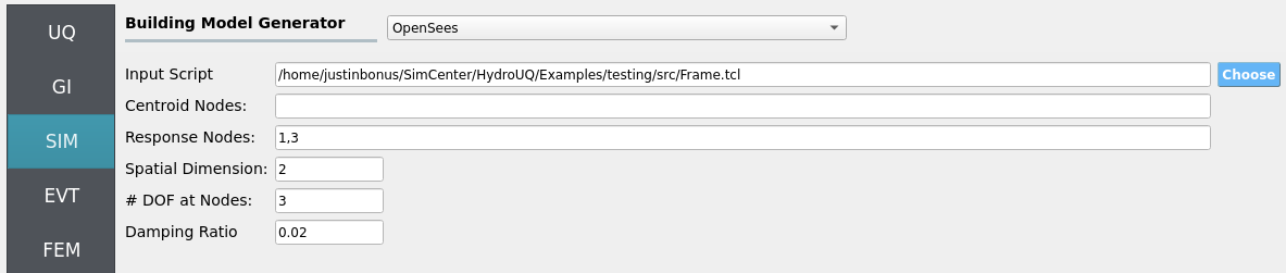
These variable names (fc, fy, E) are recognized in Frame.tcl due to use of the pset command instead of set. This is so that RV picks them up automatically. You can try adding new RV parameters in the same way.

Uncertain properties (treated as RVs; see Step 7):

• fc: mean 6, stdev 0.06

• fy: mean 60, stdev 0.6

• E: mean 30000, stdev 300

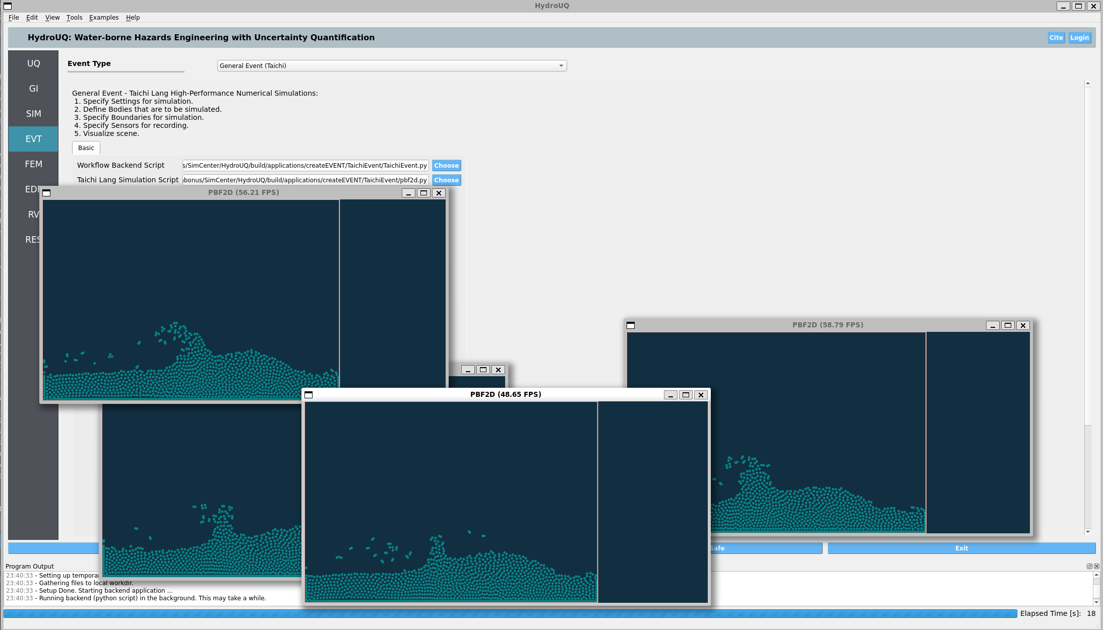
4.2.2.4. Step 4: EVT

Load Generator: Taichi Event - 2D PBFD piston wave maker (local, real-time capable).

Typical configuration (adjust to your scenario):

• Domain: width/height, particle spacing, boundary conditions (rigid walls at left/bottom; moving wall at right).

• Piston motion: stroke amplitude, frequency (or velocity profile), phase start/stop.

• PBFD numerics: solver iterations per step, CFL-safe time step, density/stiffness tuning.

• Export: per-step force/pressure sampling at the left wall; choose sampling grid/resolution and output rate.

If desired, you can promote piston parameters (e.g., amplitude/frequency) to RVs in future studies; here we keep them deterministic to focus on structural uncertainty.

You will run, and may edit to implement hydrodynamic uncertainty, the following Taichi Lang Python script for position-based fluid dynamics, pbf2d.py:

Click to expand the Python script used for this example

# Macklin, M. and Müller, M., 2013. Position based fluids. ACM Transactions on Graphics (TOG), 32(4), p.104.
# Taichi implementation by Ye Kuang (k-ye)
# Modifications for HydroUQ by Justin Bonus

import math
import os
import numpy as np

import taichi as ti

ti.init(arch=ti.gpu)

screen_res = (800, 400)
screen_to_world_ratio = 10.0
boundary = (
    screen_res[0] / screen_to_world_ratio,
    screen_res[1] / screen_to_world_ratio,
)
cell_size = 2.51
cell_recpr = 1.0 / cell_size


def round_up(f, s):
    return (math.floor(f * cell_recpr / s) + 1) * s


grid_size = (round_up(boundary[0], 1), round_up(boundary[1], 1))

dim = 2
max_frames = 1800
bg_color = 0x112F41
particle_color = 0x068587
boundary_color = 0xEBACA2
num_particles_x = 60
num_particles = num_particles_x * 20
max_num_particles_per_cell = 100
max_num_neighbors = 100
time_delta = 1.0 / 20.0
epsilon = 1e-5
particle_radius = 3.0
particle_radius_in_world = particle_radius / screen_to_world_ratio

# PBF params
h_ = 1.1
mass = 1.0
rho0 = 1.0
lambda_epsilon = 100.0
pbf_num_iters = 5
corr_deltaQ_coeff = 0.3
corrK = 0.001
# Need ti.pow()
# corrN = 4.0
neighbor_radius = h_ * 1.05

poly6_factor = 315.0 / 64.0 / math.pi
spiky_grad_factor = -45.0 / math.pi

old_positions = ti.Vector.field(dim, float)
positions = ti.Vector.field(dim, float)
velocities = ti.Vector.field(dim, float)
grid_num_particles = ti.field(int)
grid2particles = ti.field(int)
particle_num_neighbors = ti.field(int)
particle_neighbors = ti.field(int)
lambdas = ti.field(float)
position_deltas = ti.Vector.field(dim, float)
# 0: x-pos, 1: timestep in sin()
board_states = ti.Vector.field(2, float)
wall_force = ti.Vector.field(dim, float, shape=())

ti.root.dense(ti.i, num_particles).place(old_positions, positions, velocities)
grid_snode = ti.root.dense(ti.ij, grid_size)
grid_snode.place(grid_num_particles)
grid_snode.dense(ti.k, max_num_particles_per_cell).place(grid2particles)
nb_node = ti.root.dense(ti.i, num_particles)
nb_node.place(particle_num_neighbors)
nb_node.dense(ti.j, max_num_neighbors).place(particle_neighbors)
ti.root.dense(ti.i, num_particles).place(lambdas, position_deltas)
ti.root.place(board_states)


@ti.func
def poly6_value(s, h):
    result = 0.0
    if 0 < s and s < h:
        x = (h * h - s * s) / (h * h * h)
        result = poly6_factor * x * x * x
    return result


@ti.func
def spiky_gradient(r, h):
    result = ti.Vector([0.0, 0.0])
    r_len = r.norm()
    if 0 < r_len and r_len < h:
        x = (h - r_len) / (h * h * h)
        g_factor = spiky_grad_factor * x * x
        result = r * g_factor / r_len
    return result


@ti.func
def compute_scorr(pos_ji):
    # Eq (13)
    x = poly6_value(pos_ji.norm(), h_) / poly6_value(corr_deltaQ_coeff * h_, h_)
    # pow(x, 4)
    x = x * x
    x = x * x
    return (-corrK) * x


@ti.func
def get_cell(pos):
    return int(pos * cell_recpr)


@ti.func
def is_in_grid(c):
    # @c: Vector(i32)
    return 0 <= c[0] and c[0] < grid_size[0] and 0 <= c[1] and c[1] < grid_size[1]


@ti.func
def confine_position_to_boundary(p):
    bmin = particle_radius_in_world
    bmax = ti.Vector([board_states[None][0], boundary[1]]) - particle_radius_in_world
    for i in ti.static(range(dim)):
        if p[i] <= bmin:
            diff = bmin - p[i]
            if i == 0:
                ti.atomic_add(wall_force[None][i], 1000.0 * diff / time_delta)
            p[i] = bmin + epsilon * ti.random()
        elif bmax[i] <= p[i]:
            p[i] = bmax[i] - epsilon * ti.random()
    return p


@ti.kernel
def move_board():
    # probably more accurate to exert force on particles according to hooke's law.
    b = board_states[None]
    b[1] += 1.0
    period = 90
    vel_strength = 8.0
    if b[1] >= 2 * period:
        b[1] = 0
    b[0] += -ti.sin(b[1] * np.pi / period) * vel_strength * time_delta
    board_states[None] = b


@ti.kernel
def prologue():
    wall_force[None] = ti.Vector([0.0, 0.0])  # ← Clear previous step force
    # save old positions
    for i in positions:
        old_positions[i] = positions[i]
    # apply gravity within boundary
    for i in positions:
        g = ti.Vector([0.0, -9.8])
        pos, vel = positions[i], velocities[i]
        vel += g * time_delta
        pos += vel * time_delta
        positions[i] = confine_position_to_boundary(pos)

    # clear neighbor lookup table
    for I in ti.grouped(grid_num_particles):
        grid_num_particles[I] = 0
    for I in ti.grouped(particle_neighbors):
        particle_neighbors[I] = -1

    # update grid
    for p_i in positions:
        cell = get_cell(positions[p_i])
        # ti.Vector doesn't seem to support unpacking yet
        # but we can directly use int Vectors as indices
        offs = ti.atomic_add(grid_num_particles[cell], 1)
        grid2particles[cell, offs] = p_i
    # find particle neighbors
    for p_i in positions:
        pos_i = positions[p_i]
        cell = get_cell(pos_i)
        nb_i = 0
        for offs in ti.static(ti.grouped(ti.ndrange((-1, 2), (-1, 2)))):
            cell_to_check = cell + offs
            if is_in_grid(cell_to_check):
                for j in range(grid_num_particles[cell_to_check]):
                    p_j = grid2particles[cell_to_check, j]
                    if nb_i < max_num_neighbors and p_j != p_i and (pos_i - positions[p_j]).norm() < neighbor_radius:
                        particle_neighbors[p_i, nb_i] = p_j
                        nb_i += 1
        particle_num_neighbors[p_i] = nb_i


@ti.kernel
def substep():
    # compute lambdas
    # Eq (8) ~ (11)
    for p_i in positions:
        pos_i = positions[p_i]

        grad_i = ti.Vector([0.0, 0.0])
        sum_gradient_sqr = 0.0
        density_constraint = 0.0

        for j in range(particle_num_neighbors[p_i]):
            p_j = particle_neighbors[p_i, j]
            if p_j < 0:
                break
            pos_ji = pos_i - positions[p_j]
            grad_j = spiky_gradient(pos_ji, h_)
            grad_i += grad_j
            sum_gradient_sqr += grad_j.dot(grad_j)
            # Eq(2)
            density_constraint += poly6_value(pos_ji.norm(), h_)

        # Eq(1)
        density_constraint = (mass * density_constraint / rho0) - 1.0

        sum_gradient_sqr += grad_i.dot(grad_i)
        lambdas[p_i] = (-density_constraint) / (sum_gradient_sqr + lambda_epsilon)
    # compute position deltas
    # Eq(12), (14)
    for p_i in positions:
        pos_i = positions[p_i]
        lambda_i = lambdas[p_i]

        pos_delta_i = ti.Vector([0.0, 0.0])
        for j in range(particle_num_neighbors[p_i]):
            p_j = particle_neighbors[p_i, j]
            if p_j < 0:
                break
            lambda_j = lambdas[p_j]
            pos_ji = pos_i - positions[p_j]
            scorr_ij = compute_scorr(pos_ji)
            pos_delta_i += (lambda_i + lambda_j + scorr_ij) * spiky_gradient(pos_ji, h_)

        pos_delta_i /= rho0
        position_deltas[p_i] = pos_delta_i
    # apply position deltas
    for i in positions:
        positions[i] += position_deltas[i]


@ti.kernel
def epilogue():
    # confine to boundary
    for i in positions:
        pos = positions[i]
        positions[i] = confine_position_to_boundary(pos)
    # update velocities
    for i in positions:
        velocities[i] = (positions[i] - old_positions[i]) / time_delta
    # no vorticity/xsph because we cannot do cross product in 2D...


def run_pbf():
    prologue()
    for _ in range(pbf_num_iters):
        substep()
    epilogue()


def render(gui):
    gui.clear(bg_color)
    pos_np = positions.to_numpy()
    for j in range(dim):
        pos_np[:, j] *= screen_to_world_ratio / screen_res[j]
    gui.circles(pos_np, radius=particle_radius, color=particle_color)
    gui.rect(
        (0, 0),
        (board_states[None][0] / boundary[0], 1),
        radius=1.5,
        color=boundary_color,
    )
    gui.show()


@ti.kernel
def init_particles():
    for i in range(num_particles):
        delta = h_ * 0.8
        offs = ti.Vector([(boundary[0] - delta * num_particles_x) * 0.5, boundary[1] * 0.02])
        positions[i] = ti.Vector([i % num_particles_x, i // num_particles_x]) * delta + offs
        for c in ti.static(range(dim)):
            velocities[i][c] = (ti.random() - 0.5) * 4
    board_states[None] = ti.Vector([boundary[0] - epsilon, -0.0])


def print_stats():
    print("PBF stats:")
    num = grid_num_particles.to_numpy()
    avg, max_ = np.mean(num), np.max(num)
    print(f"  #particles per cell: avg={avg:.2f} max={max_}")
    num = particle_num_neighbors.to_numpy()
    avg, max_ = np.mean(num), np.max(num)
    print(f"  #neighbors per particle: avg={avg:.2f} max={max_}")


def main():
    init_particles()
    print(f"boundary={boundary} grid={grid_size} cell_size={cell_size}")
    gui = ti.GUI("PBF2D", screen_res)

    # Prepare force tracking
    force_values = []
    time_values = []

    # Output file
    force_filename = "forces.evt"
    if os.path.exists(force_filename):
        os.remove(force_filename)  # clean if it exists

    while gui.running and gui.frame < max_frames and not gui.get_event(gui.ESCAPE):
        move_board()
        run_pbf()

        # Record time and force
        current_time = gui.frame * time_delta
        time_values.append(current_time)
        fx = wall_force.to_numpy()[None][0].item(0) # x-component of the wall force
        force_values.append(fx)

        if gui.frame % 20 == 1:
            print_stats()
            print("Left wall force:", fx)

        render(gui)

    # Write to file at end
    with open(force_filename, "w") as f:
        f.write(" ".join("0.0" for _ in force_values) + "\n")
        f.write(" ".join(f"{fval:.5f}" for fval in force_values) + "\n")

if __name__ == "__main__":
    main()

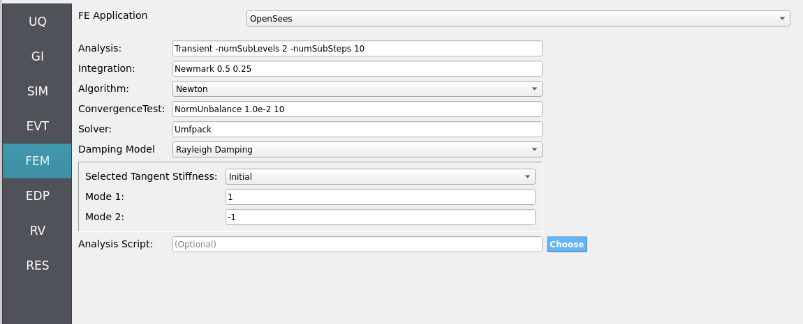
4.2.2.5. Step 5: FEM

Solver: OpenSees dynamic analysis. Check:

• Integration step compatible with PBFD export interval (or use interpolation).

• Appropriate algorithm/convergence tolerances for expected nonlinearity.

• Damping model as needed (e.g., Rayleigh).

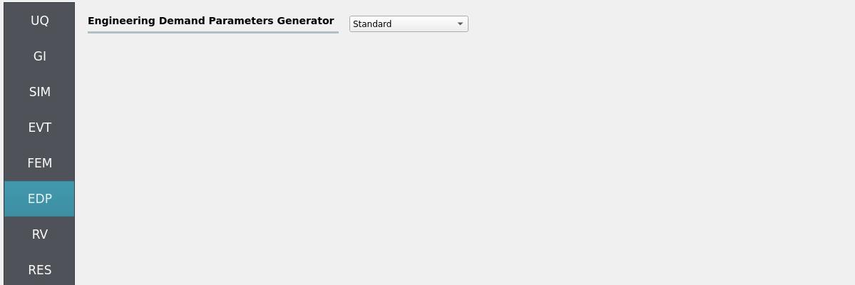
4.2.2.6. Step 6: EDP

Select Engineering Demand Parameters (EDPs) to summarize response:

• Peak Floor Acceleration (PFA)

• Root Mean Square Acceleration (RMSA)

• Peak Floor Displacement (PFD)

• Peak Interstory Drift (PID)

4.2.2.7. Step 7: RV

Define distributions for the structural RVs:

• fc: Normal (mean 6, stdev 0.06)

• fy: Normal (mean 60, stdev 0.6)

• E: Normal (mean 30000, stdev 300)

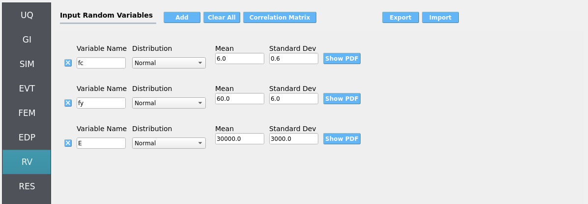
Warning

Do not leave distributions as constant when using the Dakota UQ engine unless the variable is intentionally deterministic for this study.

4.2.3. Simulation

This workflow is intended for local execution to leverage real-time/near-real-time Taichi PBFD on CPU or GPU. Click RUN. When complete, the RES panel opens.

Warning

Keep recorder counts, output frequency, and sample size reasonable. Excessive I/O (high-rate PBFD exports or too many recorders) can dominate runtime and disk usage.

We assume most modern computers will be able to run 1 - 10 of these simulations (set by samples in the UQ tab) in parallel in real-time (60 frames-per-second) or near real-time. A pop-up GUI(s) should appear once the RUN button is clicked at the bottom of the HydroUQ desktop app. The taichi PyPi will be automatically installed if your system does not currently have it. The backend graphics library is automatically swapped out by Taichi to meet your systems capabilities, though there are some edge-cases which you may contact NHERI SimCenter developers for assistance on.

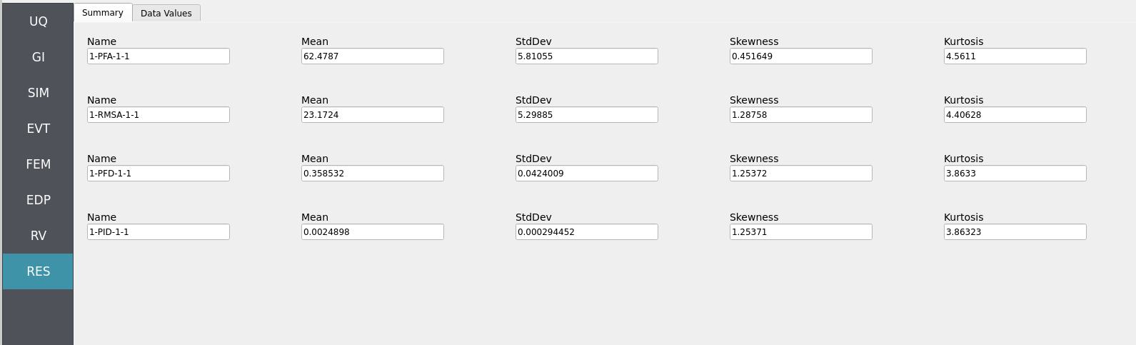
4.2.4. Analysis

Returning to our primary HydroUQ workflow, which concerns uncertainty in structural response, we may now view the final results in the RES tab. Clicking Summary on the top-bar, a statistical summary of results is shown below:

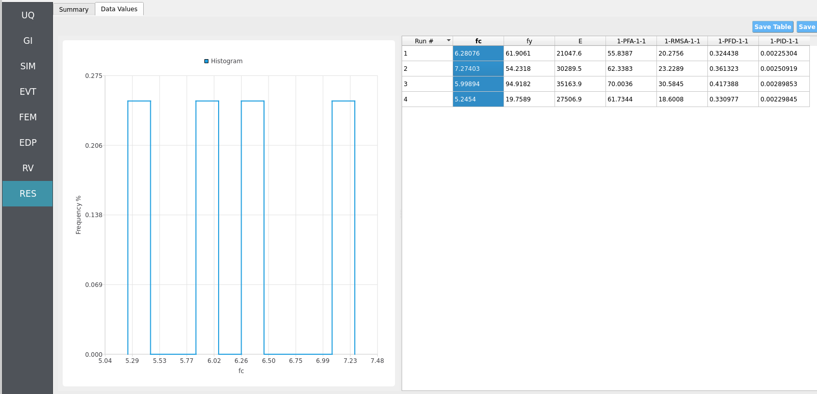
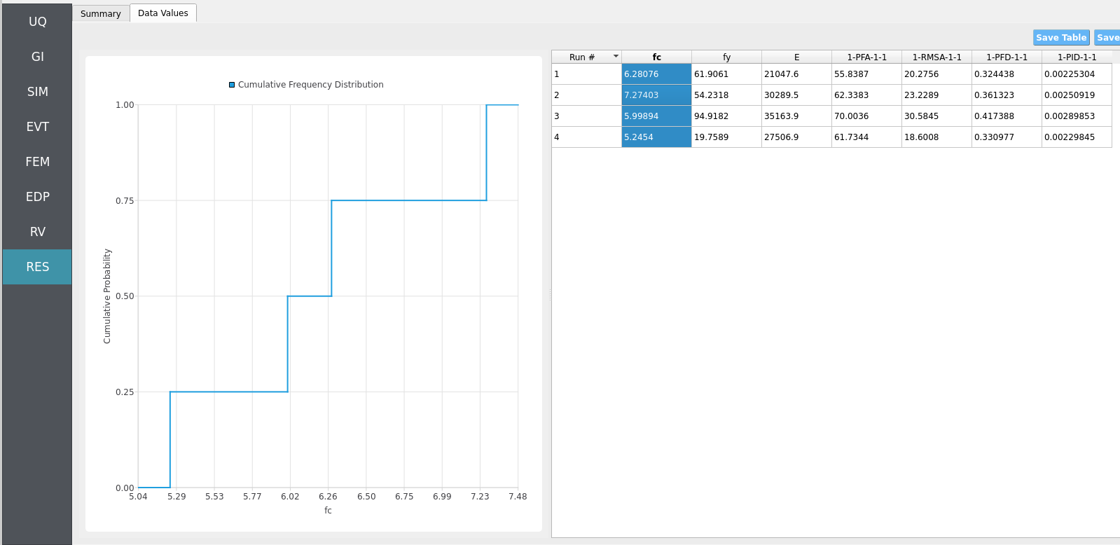
Clicking Data Values on the top-bar shows detailed histograms, cumulative distribution functions, and scatter plots relating the dependent and independent variables:

Note

In the Data Values tab, left- and right-click column headers to change plot axes; selecting a single column with both clicks displays frequency and CDF plots.

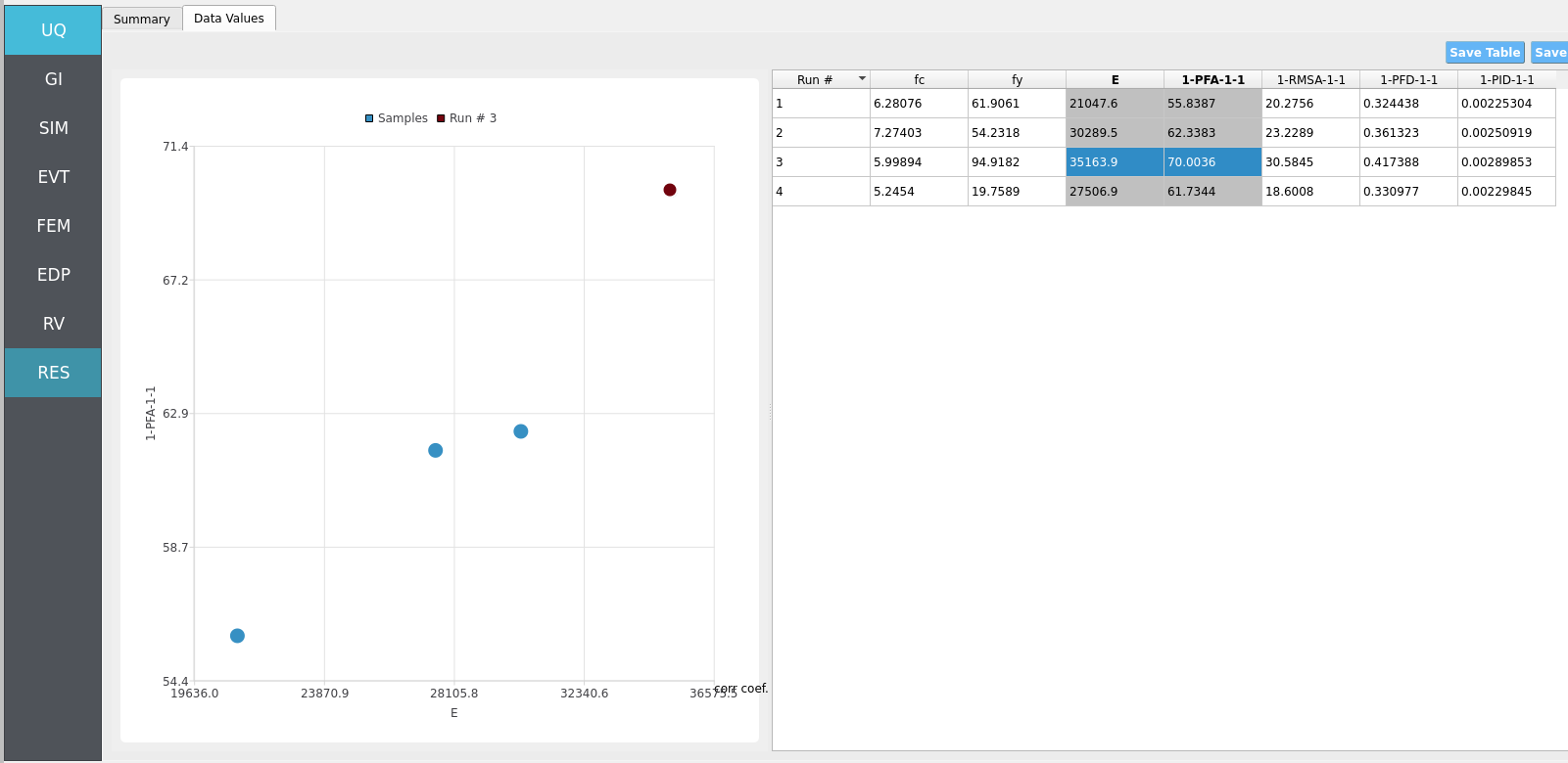
For more advanced analysis, export results as a CSV file by clicking Save Table on the upper-right of the application window. This will save the independent and dependent variable data. I.e., the Random Variables you defined and the Engineering Demand Parameters determined from the structural response per each simulation.

To save your simulation configuration with results included, click File / Save As and specify a location for the HydroUQ JSON input file to be recorded to. You may then reload the file at a later time by clicking File / Open. You may also send it to others by email or place it in an online repository for research reproducibility. This example’s input file is viewable at Reproducibility.

To directly share your simulation job and results in HydroUQ with other DesignSafe users, click GET from DesignSafe. Then, navigate to the row with your job and right-click it. Select Share Job. You may then enter the DesignSafe username or usernames (comma-separated) to share with.

Important

Sharing a job requires that the job was initially ran with an Archive System ID (listed in the GET from DesignSafe table’s columns) that is not designsafe.storage.default. Any other Archive System ID allows for sharing with DesignSafe members on the associated project. See Jobs for more details.

4.2.5. Conclusions

This example demonstrates that real-time physics simulations can be run in a modular HydroUQ workflow to determine physics-based, statistical demands on uncertain structures. Feel free to explore using Taichi Lang to simulate other scenarios and numerical methods (e.g., Smoothed Particle Hydrodynamics, Material Point Method, Finite Volume Method).

4.2.6. References

[Hu2019]

Hu, Yuanming et al. (2019). “Taichi: a language for high-performance computation on spatially sparse data structures.” ACM Transactions on Graphics (TOG). Volume 38.

4.2.7. Reproducibility

• Random seed(s): 1 (UQ/event), if reproducibility is desired

• Model file: Frame.tcl

• App version: HydroUQ v4.2.0 (or current)

• System: Local Mac, Linux, or Windows with CPU/GPU Taichi support

• Input: The HydroUQ forward sampling input file is as follows: input.json , is used:

Click to expand the HydroUQ input file used for this example

{
    "Applications": {
        "EDP": {
            "Application": "StandardEDP",
            "ApplicationData": {
            }
        },
        "Events": [
            {
                "Application": "TaichiEvent",
                "ApplicationData": {
                },
                "EventClassification": "Hydro"
            }
        ],
        "Modeling": {
            "Application": "OpenSeesInput",
            "ApplicationData": {
                "fileName": "Frame.tcl",
                "filePath": "{Current_Dir}/."
            }
        },
        "Simulation": {
            "Application": "OpenSees-Simulation",
            "ApplicationData": {
            }
        },
        "UQ": {
            "Application": "Dakota-UQ",
            "ApplicationData": {
            }
        }
    },
    "DefaultValues": {
        "driverFile": "driver",
        "edpFiles": [
            "EDP.json"
        ],
        "filenameAIM": "AIM.json",
        "filenameDL": "BIM.json",
        "filenameEDP": "EDP.json",
        "filenameEVENT": "EVENT.json",
        "filenameSAM": "SAM.json",
        "filenameSIM": "SIM.json",
        "rvFiles": [
            "AIM.json",
            "SAM.json",
            "EVENT.json",
            "SIM.json"
        ],
        "workflowInput": "scInput.json",
        "workflowOutput": "EDP.json"
    },
    "EDP": {
        "type": "StandardEDP"
    },
    "Events": [
        {
            "Application": "TaichiEvent",
            "EventClassification": "Hydro",
            "basicPyScript": "TaichiEvent.py",
            "basicPyScriptPath": "{Current_Dir}/.",
            "interfaceSurface": "pbf2d.py",
            "interfaceSurfacePath": "{Current_Dir}/."
        }
    ],
    "GeneralInformation": {
        "NumberOfStories": 1,
        "PlanArea": 129600,
        "StructureType": "RM1",
        "YearBuilt": 1990,
        "depth": 360,
        "height": 576,
        "location": {
            "latitude": 37.8715,
            "longitude": -122.273
        },
        "name": "",
        "planArea": 129600,
        "stories": 1,
        "units": {
            "force": "kips",
            "length": "in",
            "temperature": "C",
            "time": "sec"
        },
        "width": 360
    },
    "Modeling": {
        "centroidNodes": [
            1,
            3
        ],
        "dampingRatio": 0.02,
        "ndf": 3,
        "ndm": 2,
        "randomVar": [
            {
                "name": "fc",
                "value": "RV.fc"
            },
            {
                "name": "fy",
                "value": "RV.fy"
            },
            {
                "name": "E",
                "value": "RV.E"
            }
        ],
        "responseNodes": [
            1,
            3
        ],
        "type": "OpenSeesInput"
    },
    "Simulation": {
        "Application": "OpenSees-Simulation",
        "algorithm": "Newton",
        "analysis": "Transient -numSubLevels 2 -numSubSteps 10",
        "convergenceTest": "NormUnbalance 1.0e-2 10",
        "dampingModel": "Rayleigh Damping",
        "firstMode": 1,
        "integration": "Newmark 0.5 0.25",
        "modalRayleighTangentRatio": 0,
        "numModesModal": -1,
        "rayleighTangent": "Initial",
        "secondMode": -1,
        "solver": "Umfpack"
    },
    "UQ": {
        "samplingMethodData": {
            "method": "LHS",
            "samples": 4,
            "seed": 1
        },
        "parallelExecution": true,
        "saveWorkDir": false,
        "uqType": "Forward Propagation",
        "uqEngine": "Dakota"
    },
    "localAppDir": "/home/justinbonus/SimCenter/HydroUQ/build",
    "randomVariables": [
        {
            "distribution": "Normal",
            "inputType": "Parameters",
            "mean": 6,
            "name": "fc",
            "refCount": 1,
            "stdDev": 0.6,
            "value": "RV.fc",
            "variableClass": "Uncertain"
        },
        {
            "distribution": "Normal",
            "inputType": "Parameters",
            "mean": 60,
            "name": "fy",
            "refCount": 1,
            "stdDev": 10,
            "value": "RV.fy",
            "variableClass": "Uncertain"
        },
        {
            "distribution": "Normal",
            "inputType": "Parameters",
            "mean": 30000,
            "name": "E",
            "refCount": 1,
            "stdDev": 5000,
            "value": "RV.E",
            "variableClass": "Uncertain"
        }
    ],
    "remoteAppDir": "/home/justinbonus/SimCenter/HydroUQ/build",
    "resultType": "SimCenterUQResultsSampling",
    "runType": "runningLocal",
    "summary": [
    ],
    "workingDir": "/home/justinbonus/Documents/HydroUQ/LocalWorkDir"
}