4.5. Digital Wind Tunnel II: Wind Loads on Isolated Building with Simple Geometry

Problem files

weuq-0013/

This example demonstrates a Computational Fluid Dynamics (CFD) based procedure for estimating the response of a building with simple box type geometry subjected to wind loading. The example demonstrates a step-by-step process for defining the CFD model based on a target experimental setup. The target experimental model is taken from Tokyo Polytechnic University (TPU) aerodynamic database. For ease of demonstration, in this example, some simplifying assumptions are taken to model the approaching wind condition. Once the CFD simulation are completed, the recorded wind loads are applied to a 45-story building for estimating the responses.

Fig. 4.5.1 Setup of the CFD model: approaching wind, computational domain and the study building.

4.5.1. Target Experimental Measurement

Relevant geometric and flow properties taken from TPU database are provided Table 4.5.1.1 . These parameters are then specified in WE-UQ as demonstrated in Workflow. In full-scale, the study building measures 200 m high with a 40 m square plan dimension. However, for simplicity, the CFD model is created in model scale (at 1:400 geometric scale) resembling that of the experimental version.

Table 4.5.1.1 Parameters needed to define the CFD model (taken from TPU database)

Parameter	Description	Value	Unit
\(B\)	Building width	0.1	m
\(D\)	Building depth	0.1	m
\(H\)	Building height	0.5	m
\(\lambda_L\)	Geometric scale of the model	1/400
\(\lambda_V\)	Velocity scale of the model	1/4
\(\lambda_T\)	Time scale of the model	100
\(U_H\)	Roof-height mean wind speed	11.2518	m/s
\(T\)	Duration of the simulation in model scale	10	s
\(\theta\)	Wind direction	0	degrees
\(z_0\)	Aerodynamic roughness length in full scale	0.03	m
\(\rho_{air}\)	Air density	1.225	kg/m^3
\(\nu_{air}\)	Kinematic viscosity of air	\(1.5e^{-5}\)	m^2/s
\(f_{s}\)	Sampling frequency (rate)	1000	Hz

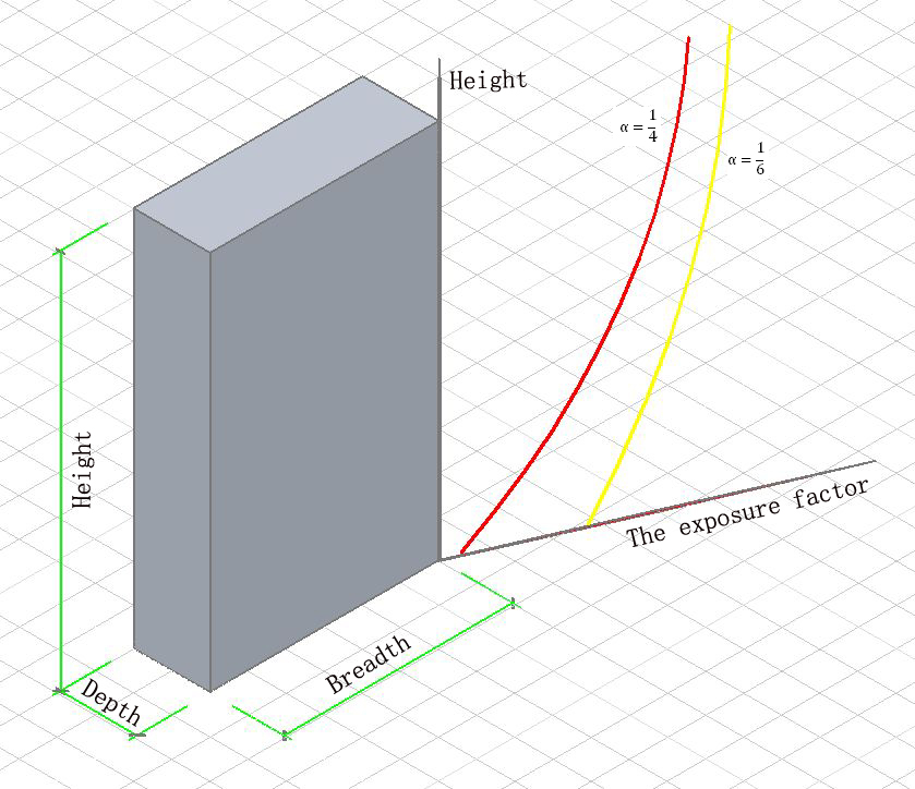
The upwind condition chosen for this example is open exposure type with a power-law coefficient \(\alpha = 1/6\), which approximately translates to a log-law aerodynamic roughness length of \(z_0 = 0.03\) m. Fig. 4.5.1.1 shows the log-law fit of the mean velocity profile extracted from the experiment. The logarithmic mean velocity profile shown in the figure is expressed by:

(4.5.1.1)\[\overline{U}(z) = \frac{u_*}{\kappa} \log\left[\frac{z-d}{z_0}\right],\]

where \(u_*\), \(\kappa = 0.4\) and \(d\) are the shear friction velocity, von Karman constant and displacement height, respectively. The value of \(d\) is set to zero, considering it is open exposure (for rough terrains it needs to be higher than 0). The shear friction velocity is determined by evaluating the log-law profile at the reference location (building height). Thus, \(u_*\) is computed as

(4.5.1.2)\[u_* = \frac{\kappa U_H}{\log(H/z_0)}.\]

As shown in Fig. 4.5.1.1, the log-law fit is reasonable for most part of the boundary layer height. However, in the upper part of the domain i.e., \(z > H(200 m)\) it shows some deviation. For cases with larger deviations from log-law, a more accurate wind profiles developed by Deaves and Harris (D&H model) need to be used ([Cook1997]). These profiles present a better description of the ABL turbulence and are also adopted in [ESDU2001] standards.

Fig. 4.5.1.1 Log-law fitting of the mean velocity profile from the experimental measurement.

Note

For ease of demonstration, in this example, the wind is assumed to a smooth flow with no significant upcoming turbulence. However, realistic wind load simulation needs to account the turbulence in the upcoming flow using appropriate inflow boundary conditions.

The experiment was run for a duration \(T = 32.768s\). But for the CFD model, considering the computational cost of running long duration simulation, we used \(T = 10s\). Also, since we used smooth inflow boundary conditions at the inlet, the wind loads will converge faster as compared to the case with a turbulent inlet. For monitoring the forces from the CFD model, we will specify the same sampling rate used in experimental measurement (\(f_{s} = 1000 Hz\)).

4.5.2. Workflow

In this example, the overall workflow is demonstrated by introducing uncertainty in the structural model. No uncertainties were considered in the wind parameters or CFD simulations. The user needs to go through the following procedure to define the Uncertainty Quantification (UQ) technique, building information, structural properties, and CFD model parameters.

Note

This example can be directly loaded from the menu bar at the top of the screen by clicking “Examples”-“E5: Wind Load Evaluation on a Generic Isolated Building Using CFD”.

4.5.2.1. UQ Method

Specify the details of uncertainty analysis in the UQ panel. This example uses forward uncertainty propagation. Select “Forward Propagation” for UQ Method and specify “Dakota” for UQ Engine driver. For the UQ algorithm, use Latin Hypercube (“LHC”). Change the number of samples to 500 and set the seed to 101.

Fig. 4.5.2.1.1 Selection of the Uncertainty Quantification Technique

4.5.2.2. General Information

Next, in the GI panel, specify the properties of the building and the unit system. For the # Stories use 50 assuming a floor height of 4 m. Set the Height, Width and Depth to 200, 40 and 40 with a Plan Area of 1600. Define the units for Force and Length as “Newtons” and “Meters”, respectively.

Warning

Note that the CFD model is created at a reduced or model scale (i.e., 1 to 400) just like the target wind tunnel model. However, the building dimensions specified here need to be in full-scale (actual building dimensions).

Fig. 4.5.2.2.1 Set the building properties in GI panel

4.5.2.3. Structural Properties

In the SIM panel, the structural properties are defined. For the structural model, select “MDOF” generator. The number of stories and floor height are automatically populated based on GI panel. For the Floor Weights put \(1.5 \times 10^7\). Replace the Story Stiffness with k to designate it as a random variable. Later the statistical properties of this random variable will be defined in RV panel. Then, input damping, yield strength, hardening ratio and other parameters as shown in Fig. 4.5.2.3.1.

Fig. 4.5.2.3.1 Define the structural properties in SIM panel

4.5.2.4. CFD Model

In the EVT panel, for the Load Generator select “CFD - Wind Loads on Isolated Building” option to create the CFD model. Here, a brief instruction to define the CFD parameters is provided. For a detailed procedure to setup the CFD model, the user is advised to refer the user manual.

1. In the Start tab, specify the path where your CFD model will be saved by clicking Browse button. It is recommended to put it in the default path i.e., Documents\WE-UQ\LocalWorkDir\IsolatedBuildingCFD. Select the Version of OpenFOAM Distribution to 9. Use the steps outlined in Modeling Process box to guide you through procedure.

   Note

   The CFD model are defined in metric system. Here after please use kilograms for Mass, meters for Length, second for Time and degrees for Angle.

Fig. 4.5.2.4.1 Setup the path and version of OpenFOAM in Start tab

2. Specify geometric details related to the building and computational domain in the Geometry tab. Set Input Dimension Normalization to Relative to size of the domain relative to the building height. Change the Geometric Scale of the CFD simulation to 1 to 400 based on the experimental setup (see Table 4.5.1.1). Set the Building Shape to Simple as the study building is a simple square building. In the Building Dimension and Orientation box specify the Wind Direction as 0 to simulate wind incidence normal to the building face. Check the COST Recommendation to automatically calculate the domain dimensions based on the COST [Franke2007] recommendations. For the coordinate system, specify the Absolute Origin as Building Bottom Center.

   Note

   If the objective is to replicate a target wind tunnel setup fully, one might need to set the Domain Length, Domain Width, Domain Height and Fetch Length manually matching the dimensions of the actual testing facility.

Fig. 4.5.2.4.2 Define the building and domain geometry in Geometry tab

3. Generate the computational grid in the Mesh tab. Follow these steps to set the mesh parameters:

   Background Mesh:

   Define the background (base) mesh as a structured grid with No. of Cells in X-axis, Y-axis and Z-axis set to 80, 40, 24. The grid size in each direction needs to be approximately the same.

   

   Fig. 4.5.2.4.3 Define the computational grid in Mesh tab

   Regional Refinements:

   Create 4 boxes to set different refinement regions using the table shown below. Each refinement box needs to have name, refinement level, min and max coordinates. Set the Level with successive increments of 1 (i.e., 1 for Box1, 2 for Box2, etc.). The Mesh Size for each region is automatically calculated and provided in the last column of the table.

   

   Fig. 4.5.2.4.4 Create regional refinements

   Surface Refinements:

   In the Surface Refinements sub-tab, check the Add Surface Refinements box. Set the Refinement Level to 6 adding an additional 2 levels of refinement from the last refinement box (Box4). These refinements are automatically applied to the building surface. For the Refinement Distance, use 0.1 which restricts the near-surface refinements within \(0.1 \times H\) distance from the building. Approx. Smallest Mesh Size gives the estimated size of the smallest mesh element(cell) near the surface of the building.

   

   Fig. 4.5.2.4.5 Create surface refinements

   Edge Refinements:

   Select Edge Refinements sub-tab and check Add Edge Refinements box. For the Refinement Level use 7 effectively making the building edges have one level finer refinement than the rest of the building surface. Similarly, the estimated smallest cell size is given in Approx. Smallest Mesh Size.

   

   Fig. 4.5.2.4.6 Apply further refinements along the building edges

   Prism Layers:

   For this example no prism layers are added. Thus, in the Prism Layers sub-tab, uncheck Add Prism Layers box. However, for more accurate CFD simulation it is recommended to have prism layers.

   

   Fig. 4.5.2.4.7 Adding Prism Layers

   Advanced Options:

   Use the default values for parameters in Advanced Options group. If you want to use more transition (buffer) cells between each refinement level, change Number of Cells Between Levels to a higher value.

   

   Fig. 4.5.2.4.8 Set Advanced Options

   Run Mesh

   Once all mesh parameters are defined, click Run snappyHexMesh button to generate the final mesh. The progress of the mesh generation can be monitored on Program Output. When the mesh generation finishes successfully, the Model View window on the right side will get updated and the user can visualize the mesh. You can actively zoom, rotate and pan the generated mesh in 3D for a detailed view. The following figure shows an inside view of the computational domain after selecting a Breakout View option in the Model View panel.

   

   Fig. 4.5.2.4.9 Running the mesh

   

   Fig. 4.5.2.4.10 Breakout View of the Mesh

4. In the Boundary Conditions tab, define properties of the approaching wind and boundary fields.

   • First, configure parameters in the Wind Characteristics group. Set the Velocity Scale to 4, the same value given in Table 4.5.1.1. The Time Scale will be automatically calculated using velocity and length scale information. Similarly, for the Wind Speed At Reference Height put \(11.25 m/s\), and set the Reference Height as building height, which is \(0.5 \, m\) in model scale. Specify the roughness of the surrounding terrain by changing Aerodynamic Roughness Length to a full-scale value of \(0.03 m\). For physical properties of the air, use \(1.225 \, kg/m^3\) for Air Density and \(1.5 \times 10^{-5} \, m^2/s\) for Kinematic Viscosity. The Reynolds number (\(Re\)) of the flow that uses the reference wind speed and height can be computed by clicking the Calculate button.

   • Then, define the boundary fields on each face of the domain including the building surface in Boundary Conditions group. At the Inlet use MeanABL which specifies a mean velocity profile based on the logarithmic profile shown in Fig. 4.5.1.1. For Outlet use a zeroPressureOutlet which sets the pressure at the outlet to zero, and helps to maintain the reference pressure in the domain around zero. On the Side and Top faces of the domain use symmetry boundary conditions. For the Ground surface, apply roughWallFunction to account for the roughness of the surrounding terrain prescribed by Aerodynamic Roughness Length (\(z_0\)). Whereas, on the Building surface, use smoothWallFunction assuming the building has a smooth surface.

   

   Fig. 4.5.2.4.11 Setup the Boundary Conditions

5. Specify turbulence modeling, solver type, duration and time step options in Numerical Setup tab.

   • For this example, since time-series of the wind forces are needed for the structural solver, we use transient CFD simulation. Thus, in Turbulence Modeling group, set Simulation Type to LES and select Smagorinsky for the Sub-grid Scale Model. The coefficients of the standard Smagorinsky model are printed in the following text box.

   • For the Solver Type select pisoFoam in Solver Selection group . Set the Number of Non-Orthogonal Correctors to 1 to add additional solver iteration. This option will give better stability to the solver as the generated mesh is non-orthogonal (irregular) near the building surface.

   • Specify \(10 s\) for the Duration of the simulation based on what is determined in Table 4.5.1.1. Compute the approximate Time Steep needed for a stable simulation by clicking Calculate button. Then, you can change the calculated time step to a slightly lower or higher value avoiding the use of long significant digits. For this example, the calculated value was \(8.67919 \times 10^{-05}\) but it was changed to \(1.0 \times 10^{-04}\) to make it a workable time step. Chose the Constant time step option.

   • Check the Run Simulation in Parallel option and specify the Number of Processors to the 32. Depending on the number of grids used, the number of processors can be increased to a higher value.

Fig. 4.5.2.4.12 Edit the Numerical Setup options

6. Select quantities of interest to record from the CFD simulation in the Monitoring tab.

   • Check Monitor Base Loads and set the corresponding Write Interval to 10, which sets the data to be written at every 10 time-step of the CFD solver.

   • The integrated story forces are always monitored as the whole workflow needs that. Similarly, here set the Write Interval to 10 which writes the story loads with a time interval of \(\Delta t \times 10 = 0.001s\). Note that this value is the same as the sampling rate (\(f_s = 1000 Hz\)) used in the experimental model. Ultimately, this is the time step the structural solver will see.

   • Uncheck the Sample Pressure Data on the Building Surface option as we only need integrated loads for this example.

   

   Fig. 4.5.2.4.13 Specify the CFD outputs in the Monitoring tab

4.5.2.5. Finite Element Analysis

To set the finite element analysis options, select the FEM panel. Here we will keep the default values as seen in Fig. 4.5.2.5.1.

Fig. 4.5.2.5.1 Setup the Finite Element analysis options

4.5.2.6. Engineering Demand Parameter

Next, select the quantity of interest from the analysis in the EDP panel. The Engineering Demand Parameters (EDPs) are structural response quantities that can be used to evaluate the performance of the structure under wind. Here select the Standard Wind EDPs which include floor displacement, acceleration and inter-story drift.

Fig. 4.5.2.6.1 Select the EDPs to measure

4.5.2.7. Random Variables

The random variables are defined in RV tab. Here, the floor stiffness named as \(k\) in SIM tab is automatically assigned as a random variable. Select Normal for the probability Distribution of the variable. Then, specify \(4 \times 10^{8}\) for the Mean and \(4 \times 10^{7}\) for Standard Dev. The user can also click Show PDF to inspect the probability density function of the variable as shown in Fig. 4.5.2.7.1

Fig. 4.5.2.7.1 Define the Random Variable (RV)

4.5.2.8. Running the Simulation

Considering the high cost of running the CFD simulation, the whole workflow can only be run remotely. Thus, once setting up the workflow is completed, the user needs to first login to DesignSafe with their credential by clicking Login button at the top right corner of the window as seen Fig. 4.5.2.8.1. Then, by pressing RUN at DesignSafe information needed for submitting the job to the remote server is specified. Put a meaningful identifier for the Job Name e.g., “TPU_LES_Example1”. Set Num Nodes to 1 and # Processes Per Node to 32. For Max Run Time, specify 17:00:00 which requests a total of 17 hours 0 minutes and 0 seconds. Finally, click the Submit button to send the job to DesignSafe

Note

We know 17 hours is a really long time!! This is quite common in most LES-based wind loads evaluation studies. If you only want to test the example, please set Duration of the simulation in Numerical Setup tab of the EVT panel to a smaller value, say \(0.1s\), and submit the simulation.

Warning

Note that the total number of processors used in the simulation equals Num Nodes \(\times\) # Processes Per Node. This value must be the same as what is specified for Number of Processors in Numerical Setup tab of the CFD model (see Fig. 4.5.2.4.12).

Warning

If the simulation cannot finish within the allocated time, it will be terminated and none of your remote simulation data can be retried. Thus, it is recommended to make Max Run Time slightly longer than what is needed to be safe.

Fig. 4.5.2.8.1 Submit the simulation to the remote server (DesignSafe-CI)

Monitor the Simulation

The progress (status) of the submitted job can be tracked by clicking GET from DesignSafe. A new window pops up showing all the jobs run on DesignSafe. Here right-click the name of your job, and select Refresh Job option to update the status of the job. If the job started the table will show RUNNING for the status. When the simulation is completed it will show FINISHED.

Fig. 4.5.2.8.2 Monitor the submitted job

4.5.2.9. Results

Once the remote job finishes, the results can be reloaded by clicking Retrieve Data option in Fig. 4.5.2.8.2. Then, the results will be displayed in RES tab. For the Standard EDP chosen the responses monitored are displayed for each floor and direction. For example, the naming of the EDPs with:

• 1-PFA-0-1: represents peak floor acceleration at the ground floor for component 1 (x-dir)

• 1-PFD-1-2: represents peak floor displacement (relative to the ground) at the 1st floor ceiling for component 2 (y-dir)

• 1-PID-3-1: represents peak inter-story drift ratio of the 3rd floor for component 1 (x-dir) and

• 1-RMSA-50-1: represents root-mean-squared acceleration of the 50th floor for component 1 (x-dir).

The four statistical moments of the EDPs which include Mean, StdDev, Skewness and Kurtosis are provided in the Summary tab of the panel.

Fig. 4.5.2.9.1 Summary of the recorded EDPs in RES panel

In addition, by switching to Data Values tab, you can see all the realizations of the simulation and inspect the relationships between different entries. For instance, if you want to visualize the variation of the top-floor acceleration with floor stiffness, right-click “1-RMSA-50-2” column in the table. This will show the root-mean-squared acceleration in the cross-wind direction for all runs as shown on the left side of Fig. 4.5.2.9.2. As you might expect, the floor acceleration generally decreases as the building becomes more stiff.

Fig. 4.5.2.9.2 (scatter-plot) Top-floor acceleration vs floor stiffness, (table) Report of EDPs for all realizations

Note

The user can interact with the plot as follows.

• Windows: left-click sets the Y axis (ordinate), while right-click sets the X axis (abscissa).

• MAC: fn-clink, option-click, and command-click all set the Y axis (ordinate). ctrl-click sets the X axis (abscissa).

4.5.3. Visualizing the CFD Output

The simulated case directory can be directly accessed on the DesignSafe data depot and visualized remotely using Paraview. The following plots show sample visualization of the instantaneous flow field.

In Fig. 4.5.3.1, the streamlines of the approaching flow, as it passes around the building, are shown. On the building surface, the result pressure coefficient are displayed. It also shows the inside view of the mesh underlying.

Fig. 4.5.3.1 Streamlines of the instantaneous velocity field around the building.

Similarly, in Fig. 4.5.3.2, the instantaneous velocity contours on the horizontal and vertical sections taken in the vicinity of the building are shown. The figure also shows the flow structure (bottom right plot) around the building. It can be seen that important flow features such as vortex shading, turbulence at the wake, and horseshoe vortex in the front of the building are captured. We recommend the user first inspect the CFD output before proceeding with results in the RES panel. This type of qualitative check constitutes the first step of verification (quality assurance) for the predicted wind loads.

Fig. 4.5.3.2 Instantaneous velocity field around the building.

Cook1997

Cook, N.J., 1997. The Deaves and Harris ABL model applied to heterogeneous terrain. Journal of wind engineering and industrial aerodynamics, 66(3), pp.197-214.

ESDU2001

ESDU, I., 2001. Characteristics of Atmospheric Turbulence Near the Ground—Part II: Single Point Data for Strong Winds (Neutral Atmosphere). Engineering Sciences Data Unit, IHS Inc., London, UK, Report No. ESDU, 85020.

TPU2005

Tokyo Polytechnic University: http://www.wind.arch.t-kougei.ac.jp/info_center/windpressure/highrise/Homepage/homepageHDF.htm

Franke2007

Franke, J., Hellsten, A., Schlünzen, K.H. and Carissimo, B., 2007. COST Action 732: Best practice guideline for the CFD simulation of flows in the urban environment.