4.9. Digital Wind Tunnel III: Wind Loads on a Building with Surroundings

Problem files

weuq-0017/

This example uses the Digital Twin capability implemented in WE-UQ Version 3.5.0. It demonstrates a Computational Fluid Dynamics (CFD) based procedure for estimating wind-induced response of a building by modeling the effect of the surroundings. The example demonstrates a step-by-step process for defining the CFD model based on a target experimental data taken from Tokyo Polytechnic University (TPU) aerodynamic database. Finally, employing the wind load generated by the CFD event, uncertainties in the structural properties such as damping are evaluated. No uncertainties were considered in the wind parameters or CFD simulations.

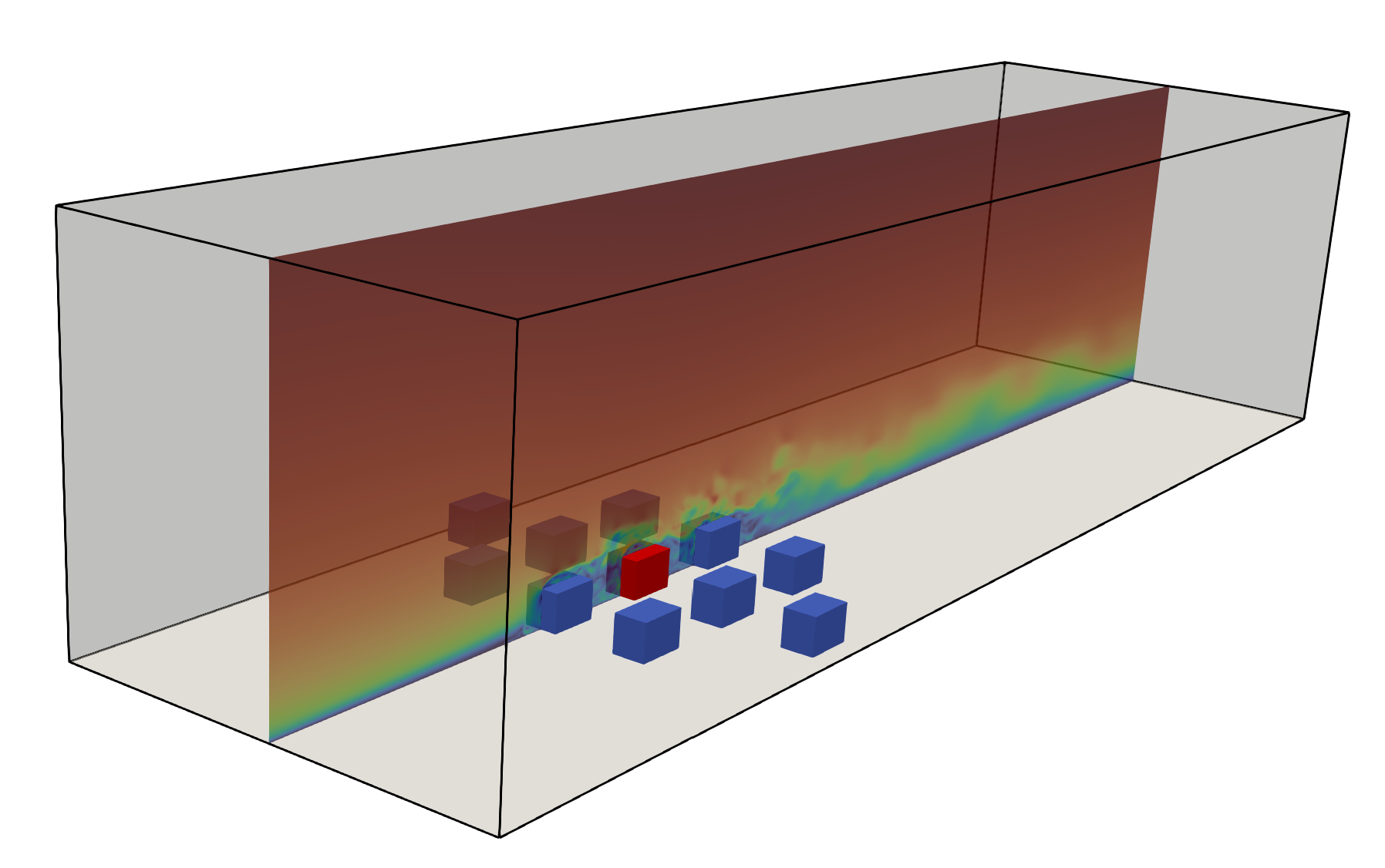
Fig. 4.9.1 Setup of the CFD model: approaching wind, computational domain, study building, and surrounding buildings.

In full-scale, the main building measures 18 m high with a 24 m x 16 m plan dimensions. For simplicity, the CFD model is created in model scale (at 1:100 geometric scale) resembling that of the experimental version. For ease of demonstration, in this example, some simplifying assumptions are taken to model the approaching wind condition. Important geometric and flow properties are provided in Table 4.9.1.

Table 4.9.1 Parameters needed to define the CFD model (taken from TPU database)

Parameter	Description	Value	Unit
\(B\)	Building width	0.16	m
\(D\)	Building depth	0.24	m
\(H\)	Building height	0.18	m
\(\lambda_L\)	Geometric scale of the model	1/100
\(\lambda_V\)	Velocity scale of the model	1/3
\(\lambda_T\)	Time scale of the model	1/33.33
\(U_H\)	Roof-height mean wind speed in model scale	8.25	m/s
\(T\)	Duration of the simulation in model scale	18.0	s
\(\theta\)	Wind direction	0	degrees
\(z_0\)	Aerodynamic roughness length in full-scale	0.3	m
\(\rho_{air}\)	Air density	1.225	kg/m^3
\(\nu_{air}\)	Kinematic viscosity of air	\(1.5e^{-5}\)	m^2/s
\(f_{s}\)	Sampling frequency (rate)	500	Hz

4.9.1. Workflow

The user needs to go through the following procedure to define the Uncertainty Quantification (UQ) technique, building information, structural properties, and CFD model parameters.

Note

This example can be directly loaded from the menu bar at the top of the screen by clicking “Examples”-“E9: Wind Load Evaluation on a Building with Surroundings using CFD”.

4.9.1.1. UQ Method

Specify the details of uncertainty analysis in the UQ panel. This example uses forward uncertainty propagation. Select “Forward Propagation” for the UQ Method and specify “Dakota” for UQ Engine driver. For the UQ algorithm, use Latin Hypercube (“LHC”). Change the number of samples to 500 and set the seed to 870.

Fig. 4.9.1.1.1 Selection of the Uncertainty Quantification Technique

4.9.1.2. General Information

Next, in the GI panel, specify the properties of the building and the unit system. For the # Stories use 6 assuming a floor height of 3 m. Set the Height, Width and Depth to 18, 16 and 24 with a Plan Area of 1600. Define the units for Force and Length as “Newtons” and “Meters”, respectively.

Warning

Note that the CFD model is created at a reduced model scale (i.e., 1 to 100) just like the target wind tunnel model. However, the building dimensions specified here need to be in full-scale (actual building dimensions).

Fig. 4.9.1.2.1 Set the building properties in GI panel

4.9.1.3. Structural Properties

In the SIM panel, the structural properties are defined. For the structural model, select “MDOF” generator. The number of stories and floor height are automatically populated based on GI panel. For the Floor Weights put \(1 \times 10^7\). Replace the Story Stiffness with \(1 \times 10^8\). Here, we assume the damping ratio to be uncertain, thus put dbg to designate it as a random variable. Later the statistical properties of this random variable will be defined in RV panel. Specify yield strength, hardening ratio and other parameters as shown in Fig. 4.9.1.3.1.

Fig. 4.9.1.3.1 Define the structural properties in SIM panel

4.9.1.4. CFD Model

In the EVT panel, for the Load Generator select “CFD - Wind Loads on Surrounded Building” option to create the CFD model. Here, a brief instruction to define the CFD parameters is provided. For a detailed procedure to setup the CFD model, the user is advised to refer the user manual.

1. In the Start tab, specify the path where your CFD model will be saved by clicking Browse button. It is recommended to put it in the default path i.e., Documents\WE-UQ\LocalWorkDir\SurroundedBuildingCFD. Use the steps outlined in Modeling Process box to guide you through procedure.

Fig. 4.9.1.4.1 Setup the path and version of OpenFOAM in the Start tab

2. Specify geometric details related to the building and computational domain in the Geometry tab. Change the Geometric Scale of the CFD simulation to 1 to 100 based on the experimental setup (see Table 4.9.1). In the Building Dimension and Orientation box specify the Wind Direction as 0 to simulate wind incidence normal width of the building. Set the length, width, height and fetch length of the domain as shown in Fig. 4.9.1.4.2 . For the surrounding buildings, use the same dimension as the study building.

Fig. 4.9.1.4.2 Define the dimensions of the computational domain, study building and surroundings in the Geometry tab

3. Generate the computational grid in the Mesh tab. Follow these steps to set the mesh parameters:

   Background Mesh:

   Create a background (base) mesh as a structured grid with No. of Cells in X-axis, Y-axis and Z-axis set to 120, 36, 30. The grid size in each direction needs to be approximately the same.

   

   Fig. 4.9.1.4.3 Define the computational grid in the Mesh tab

   Regional Refinements:

   Create 3 boxes to set different refinement regions as shown in fig-we17-EVT2. Each refinement box needs to have a name, refinement level, min and max coordinates. Set the Level with successive increments of 1 (i.e., 1 for Box1, 2 for Box2 and 3 for Box3). The Mesh Size for each region is automatically calculated and provided in the last column of the table.

Fig. 4.9.1.4.4 Create regional refinements

Surface Refinements:

In the Surface Refinements sub-tab, check the Add Surface Refinements box. Define surface refinements for the study building and the surroundings as shown in fig-we17-EVT3.

Fig. 4.9.1.4.5 Create surface refinements

Edge Refinements:

Similarly, select the Edge Refinements sub-tab and check the Add Edge Refinements box. Define edge refinements for the main and the surrounding buildings as shown bellow.

Fig. 4.9.1.4.6 Apply further refinements along the building edges

Prism Layers:

For this example, no prism layers are added. Thus, in the Prism Layers sub-tab, uncheck the Add Prism Layers box.

Run Mesh

Once all mesh parameters are defined, click the Run Final Mesh button to generate the final mesh. The progress of the mesh generation can be monitored on Program Output. When the mesh generation finishes successfully, the Model View window on the right side will get updated and the user can visualize the mesh. You can actively zoom, rotate and pan the generated mesh in 3D for a detailed view. The following figure shows an inside view of the computational domain after selecting a Breakout View option in the Model View panel.

Fig. 4.9.1.4.7 Running the mesh

Fig. 4.9.1.4.8 Breakout View of the Mesh

4. In the Boundary Conditions tab, define properties of the approaching wind and boundary fields.

   • First, configure parameters in the Wind Characteristics group. Set the Velocity Scale to 3, the same value given in Table 4.9.1. The Time Scale will be automatically calculated using velocity and length scale information. Similarly, for the Wind Speed At Reference Height put \(8.25 m/s\), and set the Reference Height as building height, which is \(0.18 \, m\) in model scale. Specify the roughness of the surrounding terrain by changing Aerodynamic Roughness Length to a full-scale value of \(0.3 m\). For physical properties of the air, use \(1.225 \, kg/m^3\) for Air Density and \(1.5 \times 10^{-5} \, m^2/s\) for Kinematic Viscosity. The Reynolds number (\(Re\)) of the flow that uses the reference wind speed and height can be computed by clicking the Calculate button.

   • Then, define the boundary fields on each face of the domain including the building surface in Boundary Conditions group. At the Inlet use MeanABL which specifies a mean velocity profile based on the logarithmic profile. For Outlet use a zeroPressureOutlet which sets the pressure at the outlet to zero, and helps to maintain the reference pressure in the domain around zero. On the Side and Top faces of the domain use symmetry boundary conditions. For the Ground surface, apply roughWallFunction to account for the roughness of the surrounding terrain prescribed by Aerodynamic Roughness Length (\(z_0\)). Whereas, on the Main Building and surrounding Buildings surface, use smoothWallFunction assuming the buildings has a smooth surface.

   

   Fig. 4.9.1.4.9 Setup the Boundary Conditions

5. Specify turbulence modeling, solver type, duration and time step options in the Numerical Setup tab.

   • For this example, since time-series of the wind forces are needed for the structural solver, we use transient CFD simulation. Thus, in Turbulence Modeling group, set Simulation Type to LES and select Smagorinsky for the Sub-grid Scale Model. The coefficients of the standard Smagorinsky model are printed in the following text box.

   • For the Solver Type select pimpleFoam in Solver Selection group . Set the Number of Non-Orthogonal Correctors to 1 to add additional solver iteration. This option will give better stability to the solver as the generated mesh is non-orthogonal (irregular) near the buildings surface.

   • Specify \(19.0 s\) for the Duration of the simulation based on what is determined in Table 4.9.1. Since we are using pimpleFoam solver, check Adjustable for time step. Compute the approximate Time Steep needed for a stable simulation by clicking Calculate button. Then, you can change the calculated time step to a slightly lower or higher value avoiding the use of long significant digits. For this example, the calculated value was \(0.00365867\) but it was changed to \(0.0025\) to be safe. For the Maximum Courant Number use 4.

   • Check the Run Simulation in Parallel option and specify the Number of Processors to the 96. Depending on the number of grids used, the number of processors can be increased to a higher value.

Fig. 4.9.1.4.10 Edit the Numerical Setup options

6. Select quantities of interest to record from the CFD simulation in the Monitoring tab.

   • The integrated story forces are always monitored as the whole workflow needs that. Similarly, here set the Write Interval to 2 which writes the story loads with a time interval of \(\Delta t \times 2 = 0.005s\). Note that this value is the same as the sampling rate (\(f_s = 500 Hz\)) used in the experimental model. Ultimately, this is the time step the structural solver will take.

   

   Fig. 4.9.1.4.11 Specify the CFD outputs in the Monitoring tab

4.9.1.5. Finite Element Analysis

To set the finite element analysis options, select the FEM panel. Here we will keep the default values as seen in Fig. 4.9.1.5.1.

Fig. 4.9.1.5.1 Setup the Finite Element analysis options

4.9.1.6. Engineering Demand Parameter

Next, select the quantity of interest from the analysis in the EDP panel. The Engineering Demand Parameters (EDPs) are structural response quantities that can be used to evaluate the performance of the structure under wind. Here select the Standard Wind EDPs which include floor displacement, acceleration and inter-story drift.

Fig. 4.9.1.6.1 Select the EDPs to measure

4.9.1.7. Random Variables

The random variables are defined in the RV tab. Here, the damping ratio named as \(dgp\) in SIM tab is automatically assigned as a random variable. Select Normal for the probability Distribution of the variable. Then, specify \(0.02\) for the Mean and \(0.004\) for Standard Dev. The user can also click Show PDF to inspect the probability density function of the variable as shown in Fig. 4.9.1.7.1

Fig. 4.9.1.7.1 Define the Random Variable (RV)

4.9.1.8. Running the Simulation

Considering the high cost of running the CFD simulation, the whole workflow can only be run remotely. Thus, once setting up the workflow is completed, the user needs to first login to DesignSafe with their credential by clicking Login button at the top right corner of the window as seen Fig. 4.9.1.8.1. Then, by pressing RUN at DesignSafe information needed for submitting the job to the remote server is specified. Put a meaningful identifier for the Job Name e.g., “TPU_LES_Surrounded”. Set Num Nodes to 2 and # Processes Per Node to 48. For Max Run Time, specify 12:00:00 which requests a total of 12 hours 0 minutes and 0 seconds. Finally, click the Submit button to send the job to DesignSafe

Warning

Note that the total number of processors used in the simulation equals Num Nodes \(\times\) # Processes Per Node. This value must be the same as what is specified for the Number of Processors in the Numerical Setup tab of the CFD model (see Fig. 4.9.1.4.10).

Fig. 4.9.1.8.1 Submit the simulation to the remote server (DesignSafe-CI)

Monitor the Simulation

The progress (status) of the submitted job can be tracked by clicking GET from DesignSafe. A new window pops up showing all the jobs run on DesignSafe. Here right-click the name of your job, and select the Refresh Job option to update the status of the job. If the job started the table will show RUNNING for the status. When the simulation is completed it will show FINISHED.

Fig. 4.9.1.8.2 Monitor the submitted job

4.9.1.9. Results

Once the remote job finishes, the results can be reloaded by clicking the Retrieve Data option in Fig. 4.9.1.8.2. Then, the results will be displayed in the RES tab. For the Standard EDP chosen the responses monitored are displayed for each floor and direction. For example, the naming of the EDPs with:

• 1-PFA-0-1: represents peak floor acceleration at the ground floor for component 1 (x-dir)

• 1-PFD-1-2: represents peak floor displacement (relative to the ground) at the 1st floor ceiling for component 2 (y-dir)

• 1-PID-3-1: represents peak inter-story drift ratio of the 3rd floor for component 1 (x-dir) and

• 1-RMSA-6-1: represents root-mean-squared acceleration of the 6th floor for component 1 (x-dir).

The four statistical moments of the EDPs which include Mean, StdDev, Skewness and Kurtosis are provided in the Summary tab of the panel.

Fig. 4.9.1.9.1 Summary of the recorded EDPs in RES panel

In addition, by switching to the Data Values tab, you can see all the realizations of the simulation and inspect the relationships between different entries. For instance, if you want to visualize the variation of the top-floor acceleration with floor stiffness, right-click the “1-RMSA-6-2” column in the table. This will show the root-mean-squared acceleration in the cross-wind direction for all runs as shown on the left side of Fig. 4.9.1.9.2. As you might expect, the floor acceleration generally decreases as the building becomes more stiff.

Fig. 4.9.1.9.2 (scatter-plot) Top-floor acceleration vs floor stiffness, (table) Report of EDPs for all realizations

Note

The user can interact with the plot as follows.

• Windows: left-click sets the Y axis (ordinate), while right-click sets the X axis (abscissa).

• MAC: fn-clink, option-click, and command-click all set the Y axis (ordinate). ctrl-click sets the X axis (abscissa).

4.9.2. Visualizing the CFD Output

Once the results are retried the simulated case directory can be directly accessed from the local case directory given in Start tab of the EVT panel. The following videos show sample visualization of the instantaneous flow field.