4.3. Wind Tunnel-Informed Stochastic Wind Load Generation

Problem files

weuq-0012/

This example estimates the probabilistic response of a building model excited by wind tunnel-informed stochastic wind loads. This example uses the experimental data obtained at the University of Florida (UF) NHERI Experimental Facility (EF), and applies the simulated wind loads to a 25-story rectangular shaped building model for response simulation.

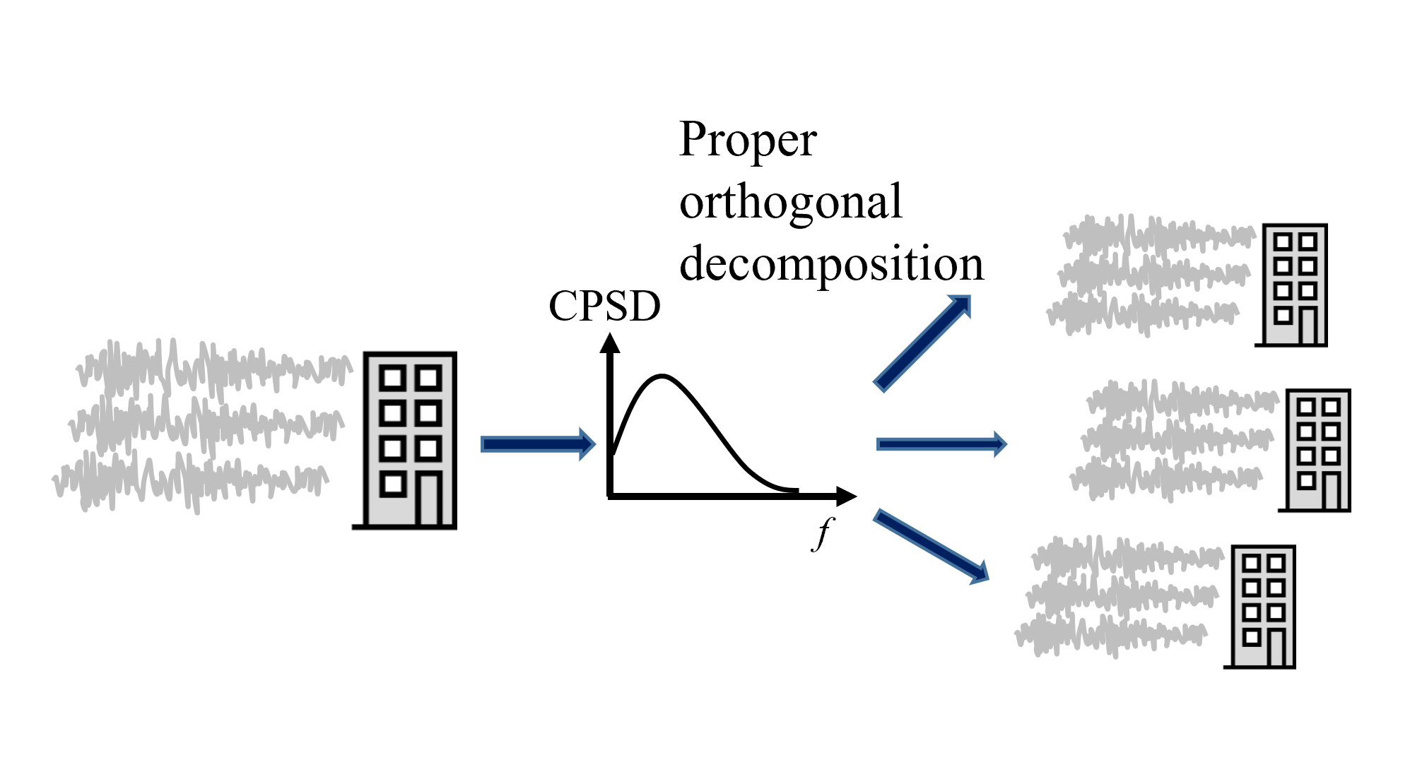
Fig. 4.3.1 Generating full-scale wind force time series from a model-scale wind force time series obtained from wind tunnel experiments.

This example uses the data presented in [Duarte2023].

Duarte2023(1,2,3)

Duarte, T.G., Arunachalam, S., Subgranon, A. and Spence, S.M., (2023). Uncertainty Quantification and Simulation of Wind-Tunnel-Informed Stochastic Wind Loads. Wind, 3(3), pp.375-393.

4.3.1. Preparation of “Wind Force Time History File”

The experimental records should first be reformatted by the user such that wind force time histories recorded at each floor in x-, y-, and z- directions (Fx, Fy, and Tz, respectively) can be directly imported in WE-UQ in the EVT tab. The dataset can be imported as either a MATLAB binary file or a json file. Additionally, the model-scale dimensions and additional information on the experiment should be provided. Please refer to the User Manual for the list of variables the file should contain. In this example, the variables in the table below are imported as a json file. Note that the x- and y- directional forces and z-directional moments at each of the 25 stories are recorded for 32 sec with dt=0.0016 sec (20,000 time points). The reference wind speed (Vref) was measured at top of the building model.

Table 4.3.1.1 Variables imported to WE-UQ

Variable	Values	Units
B	0.3	m
D	0.6	m
H	0.5	m
fs	625	Hz
Vref	12.25	m/s
Fx	[25x20000] array	N
Fy	[25x20000] array	N
Tz	[25x20000] array	N·m
t	[1x20000] array	sec

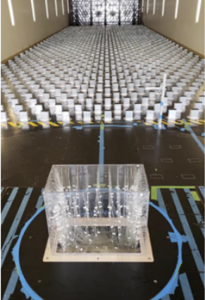
Fig. 4.3.1.1 The experiment was performed at UF [Duarte2023].

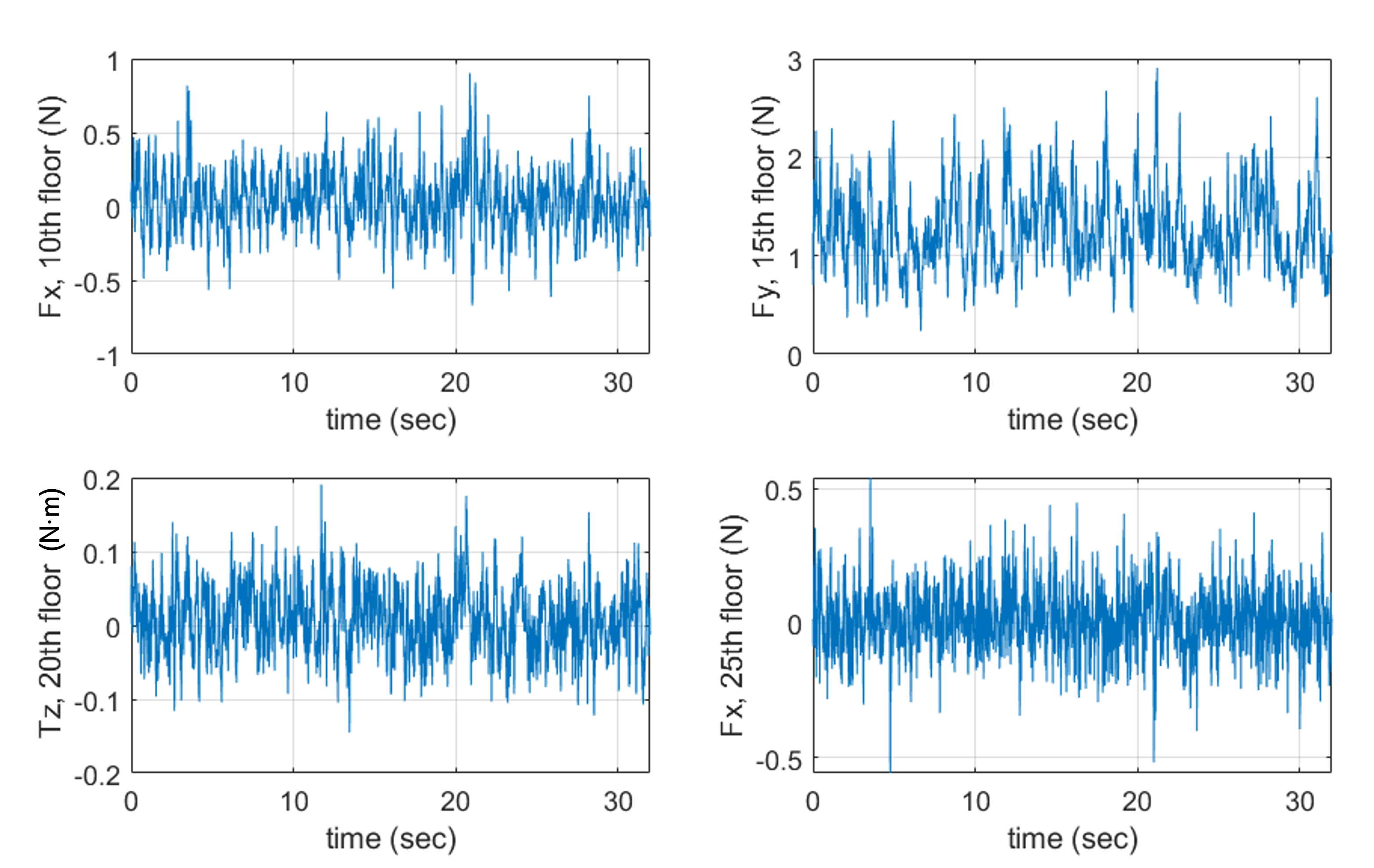
Fig. 4.3.1.2 Examples of Wind Force Time Series in Fx, Fy, Tz arrays [Duarte2023].

The json file used in this example is named Forces_ANG000_phase1.json, and it can be found at weuq-0012/src. Using this information, WE-UQ will generate the stochastic wind loads that apply to a full-scale building model with scaling factor of 200.

4.3.2. Workflow

Note

This example can be directly loaded from the menu bar at the top of the screen by clicking “Examples”-“E4: Wind Tunnel-Informed Stochastic Wind Load Generation”. The user may want to increase the number of samples in the UQ tab for more stable results.

1. In the UQ tab, click “forward propagation” to perform Monte Carlo simulation. Set the number of samples 50.

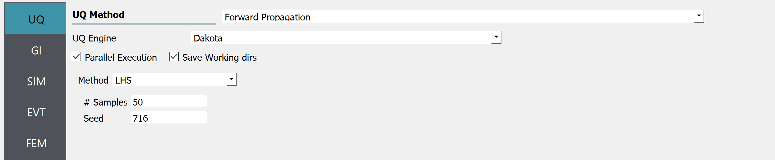
Fig. 4.3.2.1 UQ tab

2. In the GI tab, set # Stories 25 as our dataset is for a 25-story building. Multiply the building scaling factor 200 by the model dimensions (0.5m x 0.3m x 0.6m; this information should be imported in “Wind Force Time History File” at the EVT tab as shown in the previous section) and specify the full-scale building dimension at Height, Width, and Depth, which respectively are 100, 60, and 120. Define the Force and Length Units of Newtons and Meters.

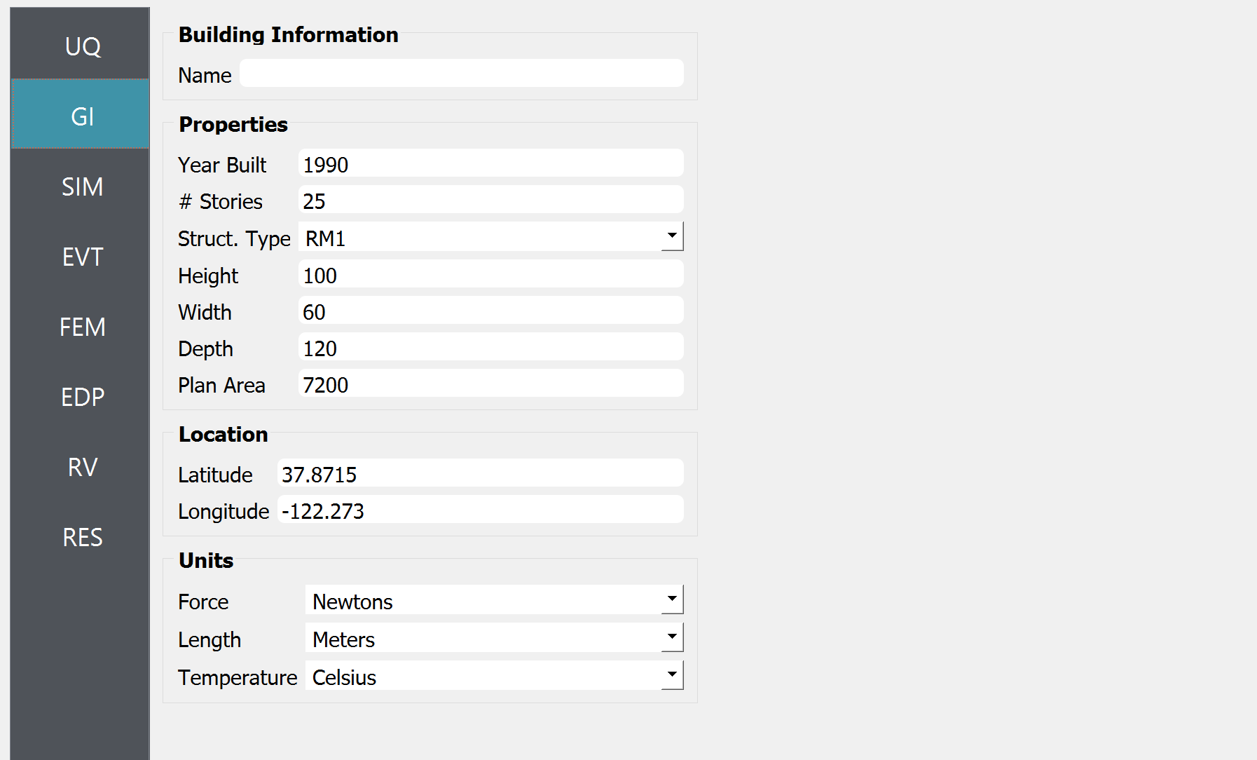
Fig. 4.3.2.2 GI tab

3. In the SIM tab, the building properties are specified. We used the floor weights of 1.e7 across the floors, and the stiffness values in each story are given as

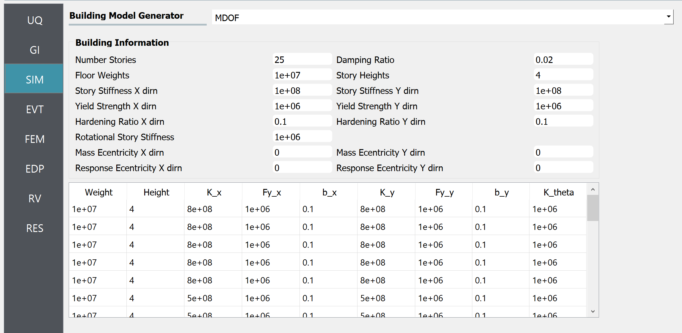
Fig. 4.3.2.3 SIM tab

Table 4.3.2.1 Stiffness of the structure

Floors	Stiffness
1-5	8.e8
6-11	5.e8
12-14	4.e8
15-17	3.e8
18-19	2.5e8
20-21	1.7e8
20-21	1.7e8
22-24	1.2e8
25	0.7e8

4. In the EVT tab, select the “Experimental Wind Forces” option for the Load Generator. Let us consider 25% of modes for the principal orthogonal decomposition (POD). The Full Scale Reference Wind Speed at the top of the building is set 30 m/s. The duration of the generated wind loads is set to 1600 sec. The “Wind Force Time History File” shown in the previous section is imported next. The model scale is auto-populated only if the datasets are provided in a json file (instead of a matlab binary file). For estimating the cross-power spectrum density function (CPSD), a window size of 4 sec, and an overlap percentage of 50 % are used. Please refer to the user manual for more details of those parameters.

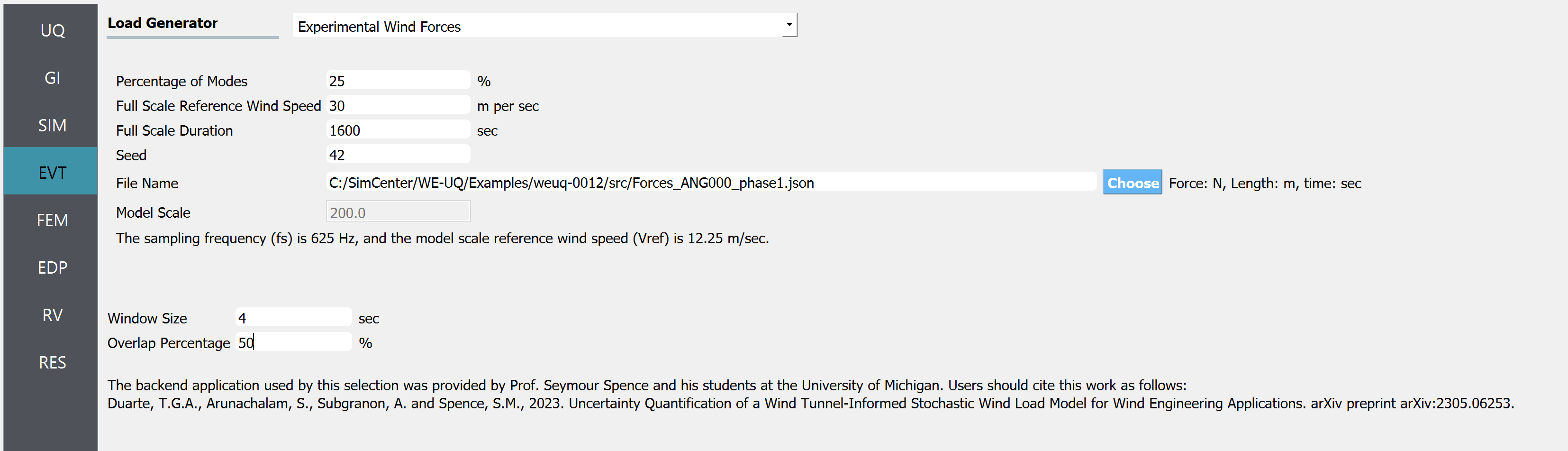
Fig. 4.3.2.4 EVT tab

5. The FEM and EDP tabs are kept as default. Under the Standard Wind EDP, in this example, the structural model will automatically output peak floor acceleration (PFA), peak floor displacement respective to the ground (PFD), Peak inter-story drift ratio (PID), root-mean-squared acceleration (RMSA).

6. In the RV tab, only a dummy variable that is not used in the UQ analysis is specified. This is because, in this example, we are only interested in the uncertainty (stochasticity) that arises in the wind load time histories.

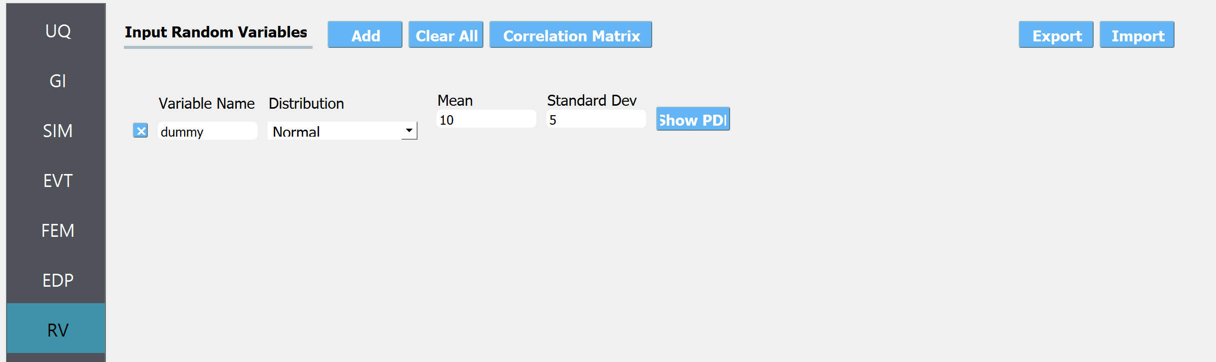
Fig. 4.3.2.5 RV tab

Note

The user can additionally specify random variables for structural parameters by putting a string for some of the structural properties in GI tab (e.g. “W” for the floor weight instead of 1.e7), and specifying the corresponding probability distribution at the RV tab (e.g. name: W, distribution: Normal, Mean: 1.e7, Standard Dev: 1.e6).

7. Once all the information is provided, click the Run or Run at DesignSafe button to run the analysis.

4.3.3. Results

Once the analysis is done, the sampling results will be displayed in the RES tab. Note that the EDP name consists of the quantity of interest, story number, and the direction of interest - for example:

• 1-PFA-0-1 : peak floor acceleration at the ground floor, component 1 (x-dir)

• 1-PFD-1-2 : peak floor displacement (respective to the ground) at the 1st floor ceiling, component 2 (y-dir)

• 1-PID-3-1 : peak inter-story drift ratio of the 3rd floor, component 1 (x-dir)

• 1-RMSA-10-1 : root-mean-squared acceleration of the 10th floor, component 1 (x-dir)

The response statistics are first displayed.

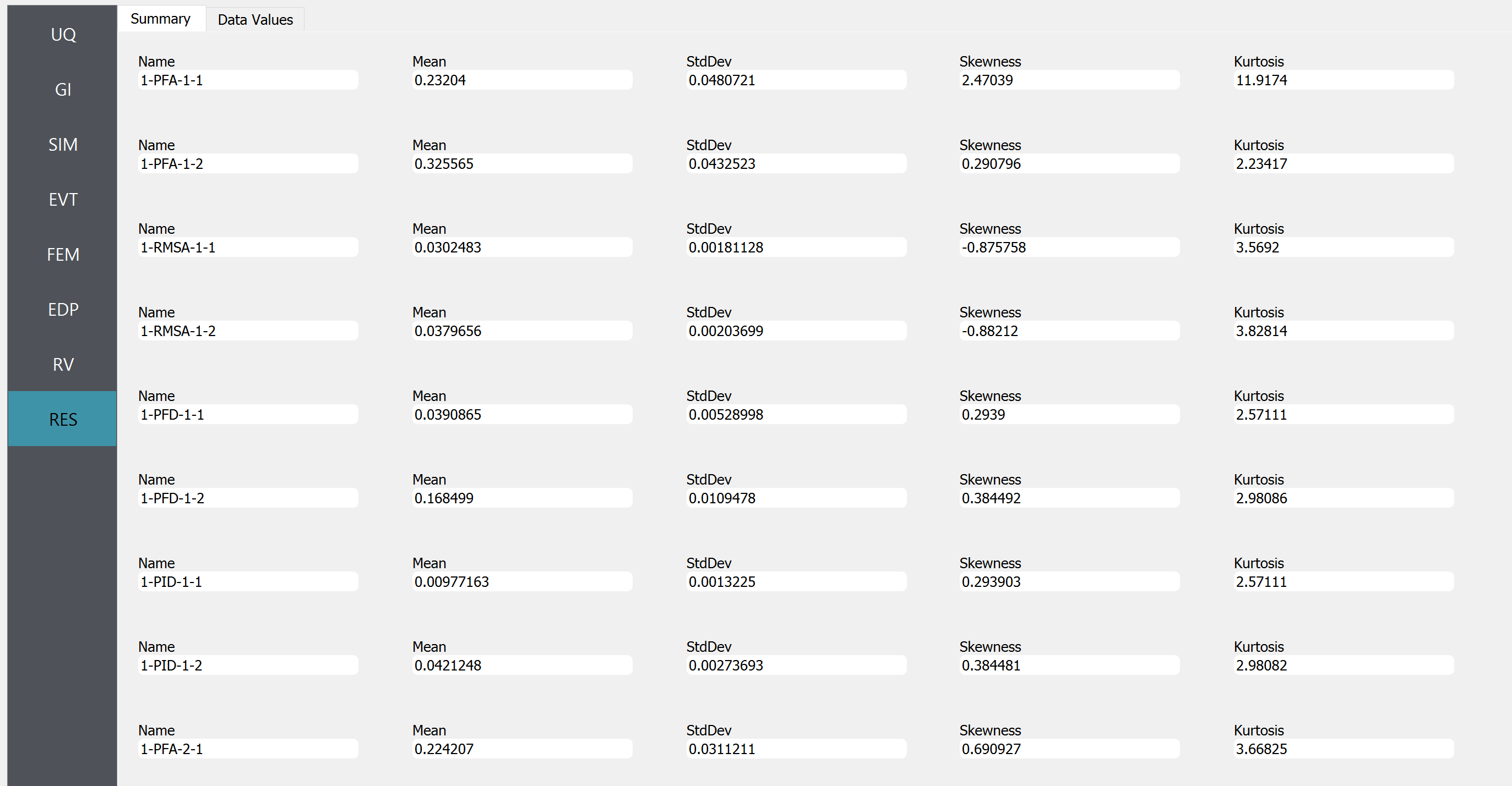
Fig. 4.3.3.1 RES tab - statistics

Additionally, the user can browse the sample realization values and inspect the correlation between various components.

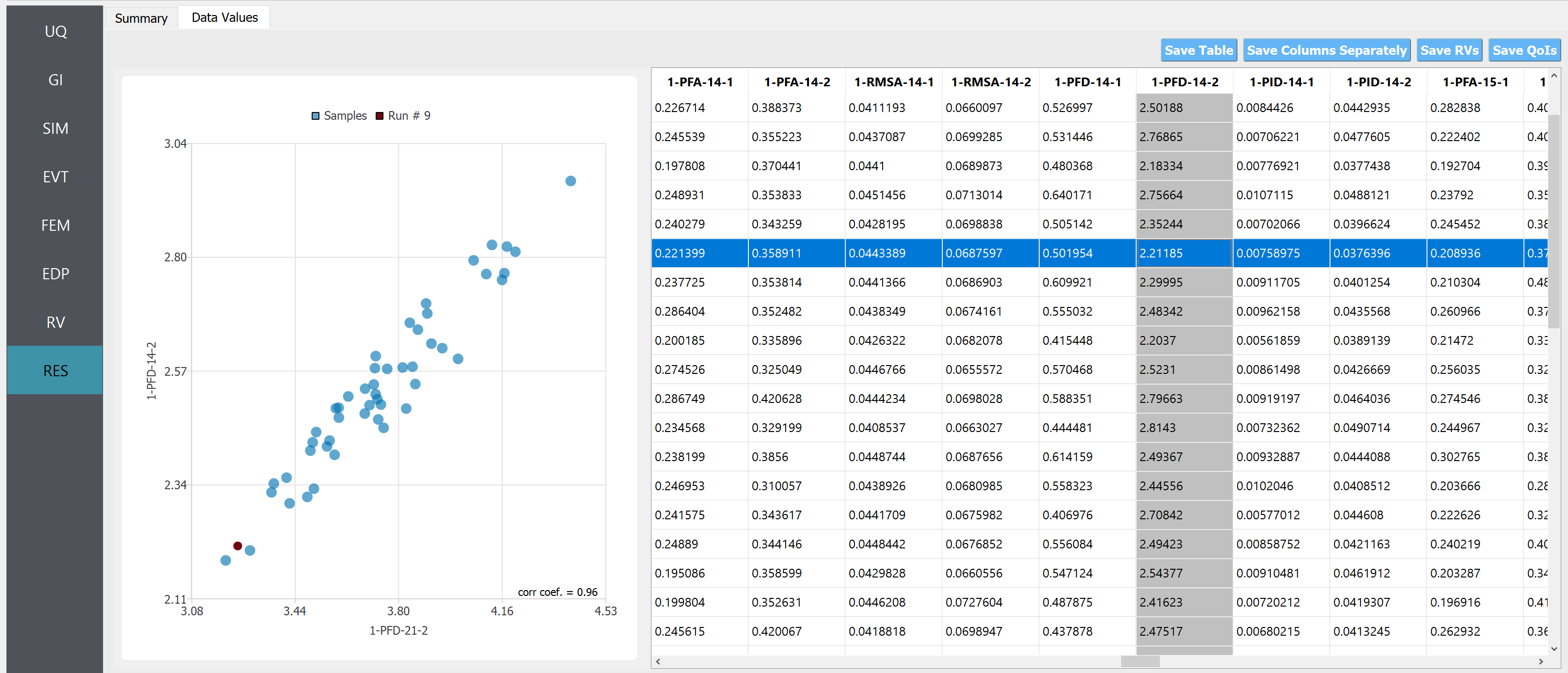
Fig. 4.3.3.2 RES tab - scatter plots

Note

The user can interact with the plot as follows.

• Windows: left-click sets the Y axis (ordinate). right-click sets the X axis (abscissa).

• MAC: fn-clink, option-click, and command-click all set the Y axis (ordinate). ctrl-click sets the X axis (abscissa).