3.1. Interpoint Distances¶

This is not a structural example, it is one used in the literature to verify sampling methods as a mathematical formula exists for the solution. The example presented is computing the average distance between randomly chosen points in a rectangular region. Such average distances come up in many settings. For cell phone companies, the probability that a distributed network is fully connected depends on average distances between communicating nodes. For city planners preparing for disasters, it could represent the average distances from dwellings to fire stations or from the dwellings to the epicenter of an earthquake.

The problem is defined as follows: Suppose two points \(P\) and \(Q\) are independent and considered uniformly distributed random points in a finite rectangle of dimension \(L_w\) and \(L_h\). It has been shown that the expected average distance between these two points \(E(P,Q)\) is given by the formula:

(3.1.1)¶\[E(P,Q) = \frac{1}{15} \left( \frac{L_w^3}{L_h^2}+\frac{L_h^3}{L_w^2}+d\left(3-\frac{L_w^2}{L_h^2}-\frac{L_h^2}{L_w^2}\right) +\frac{5}{2} \left(\frac{L_h^2}{L_w}\log\right(\frac{L_w+d}{L_h}\left)+\frac{L_w^2}{L_h}\log\left(\frac{L_h+d}{L_w}\right)\right)\right)\]

where \(d=\sqrt{L_w^2+L_h^2}\)

Using the above formula one can compute a number of expected distances for rectangles of different sizes, for example:

Lw	Lh	E
1.0	0.6	0.4239
2.0	0.8	0.7651
10.0	7.5	4.5865
10.0	10.0	7.7502

Note

The above table was computed using the following Matlab script, run repeatedly for different values of Lw and Lh.

Lw = 1.0
Lh = 0.6
d = sqrt(Lh^2+Lw^2)
E = 1/15*(Lw^3/Lh^2 + Lh^3/Lw^2 + d * (3- Lw^2/Lh^2 - Lh^2/Lw^2) + 5/2 * (Lh^2/Lw * log((Lw+d)/Lh) + Lw^2/Lh * log((Lh+d)/Lw)))

In the following steps we will demonstrate how this is done using the quoFEM app with figures showing the inputs for case with Lw=1.0, Lh= 0.6 and utilizing LHS with 1000 samples. A table will provide additional results for other sampling methods and numbers of samples.

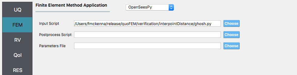
Repeating this exercise in quoFEM requires using either the OpenSees or the OpenSeesPy Interpreter. Depending on your choice, create a new folder and in it place one of the following files, the first is a Python script to be named ghosh.py. It is to be used with the OpenSeesPy FEM application.

import math

x1 = "RV.x1"
y1 = "RV.y1"
x2 = "RV.x2"
y2 = "RV.y2"

D = math.sqrt((x2-x1)*(x2-x1)+(y2-y1)*(y2-y1))

f = open("results.out", "w")
f.write(str(D))
f.close()

The second a tcl script to be named ghosh.tcl. It is to be used with the OpenSees FEM application.

# note: the variables x1, y1, x2, y2 will be provided when runs in workflow
# as long as they are defined as random variables

set D [expr sqrt(($x2-$x1)*($x2-$x1)+($y2-$y1)*($y2-$y1))]

set f [open "results.out" "w"]
puts $f $D
close $f

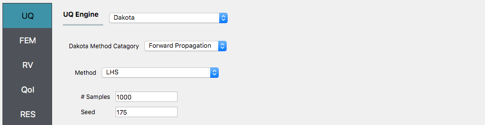
Start the quoFEM app and select Dakota UQ Engine, Forward propagation type of problem and LHS method. Specify 10000 samples and a seed of 175.

Select next the FEM tab. From this tab select either OpenSees or OpenSeesPy depending on which file you choose to place in the folder. For the input file specify the full path to this file.

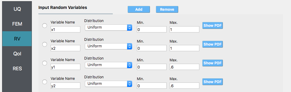
Select the RV tab. Create four random variables named X1, Y1, X2, Y2. For each specify a uniform distribution with the range for the X variables being 0 and Lw and range of Y variables being 0 and Lh. This is as shown for Lw = 1.0 and Lh = 0.6.

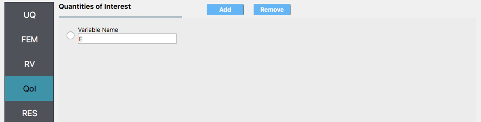
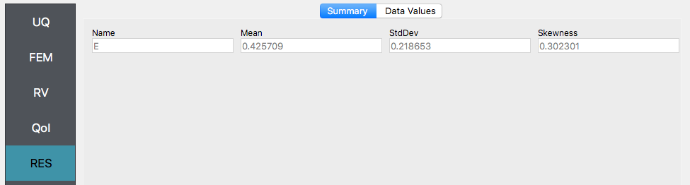
Select the QoI tab. Create one EDP and name it E as shown.

Press the Run button. The results should show the mean to be 0.425709.

These simulations can be performed for a number of the different sampling methods for a number of different number of samples.

Method	#Samples	E(P,Q)	Error
MC	100	0.447626	0.0560
MC	1000	0.430936	0.0166
MC	10000	0.421910	0.0047
LHS	100	0.435349	0.0270
LHS	1000	0.425709	0.0043
LHS	10000	0.422350	0.0037