2. Getting Started Tutorial¶

2.1. Before We Start¶

If you have not yet installed quoFEM, please see

Install quoFEM

Run quoFEM without installation

Important

If you just downloaded quoFEM, but have previously used the older version of it or other SimCenter tools, it is recommended to reset the cached path values by pressing the reset button in File-Preference.

2.2. quoFEM for a Python Model Interface¶

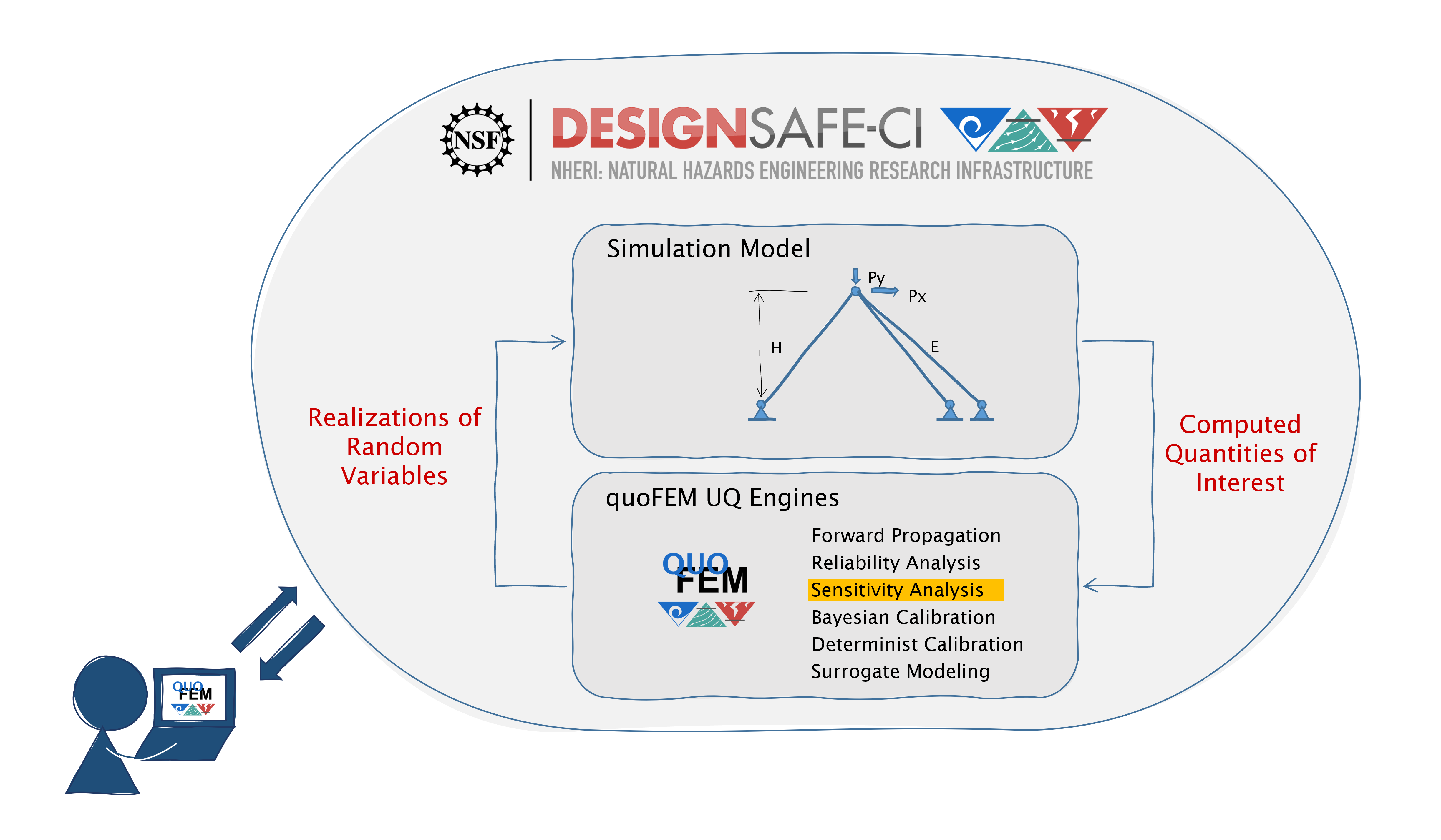
This tutorial will show how a deterministic model written/interfaced in a Python script can be used for Uncertainty Quantification analysis, using an example of global sensitivity analysis.

Step 0. Prepare a Python Model

Step 1. Modify the Model Script to Define Random Variables and Quantities of Interest

Step 2. Run quoFEM

Step 3. Run quoFEM at DesignSafe

Step 0

Step 0. Prepare a Python Model

Let us grab a python script from OpenSeesPy example manual for this tutorial. Please follow the steps:
In OpenSeesPy example manual, navigate to Structural Example - Elastic Truss Analysis

In the Elastic Truss Analysis page, click the download button. Create a new folder named TrussExample and save ElasticTruss.py in the folder.

Fig. 2.2.1 Download OpenSeesPy Elastic Truss Analysis¶

Important

It is important to save the model in a new folder instead of root, desktop or downloads

Test Your Model Test if the input script ElasticTruss.py runs successfully using the command prompt (Windows) or terminal (Mac). To do this, navigate into TrussExample folder using cd command and type the following.
{$PathToPythonExe} ElasticTruss.py
where {$PathToPythonExe} should be replaced with the python path found in the preference window.

Fig. 2.2.2 Find the Python path in File-Preference in the menu bar¶

According to ElasticTruss.py, the analysis should print out “Passed!”, meaning the model ran successfully.

Fig. 2.2.3 Testing ElasticTruss.py¶

Now we are ready to run a probabilistic analysis using this model.
Note

openseespy, numpy and matplotlib libraries are readily available in quoFEM because:

Windows
quoFEM is bundled with a Python executable which has those packages pre-installed. See here.

macOS
In the installation steps, the command pip3 install nheri_simcenter --upgrade will include those packages

It is important to test the model using the “correct” Python executable the quoFEM uses, which is that shown in the preference. See here to read more on Python versions and installing additional packages.

Step 1

Step 1. Modify the Model Script to Define Random Variables and Quantities of Interest

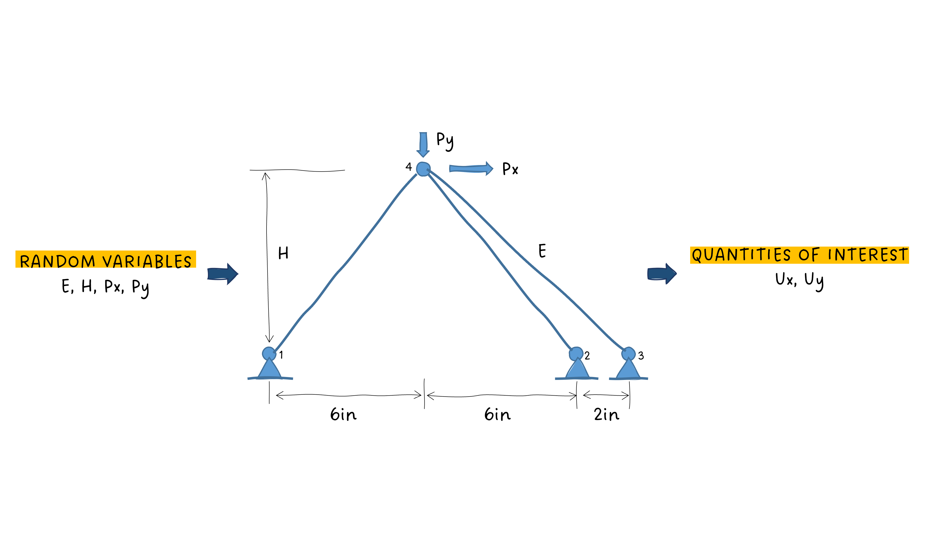
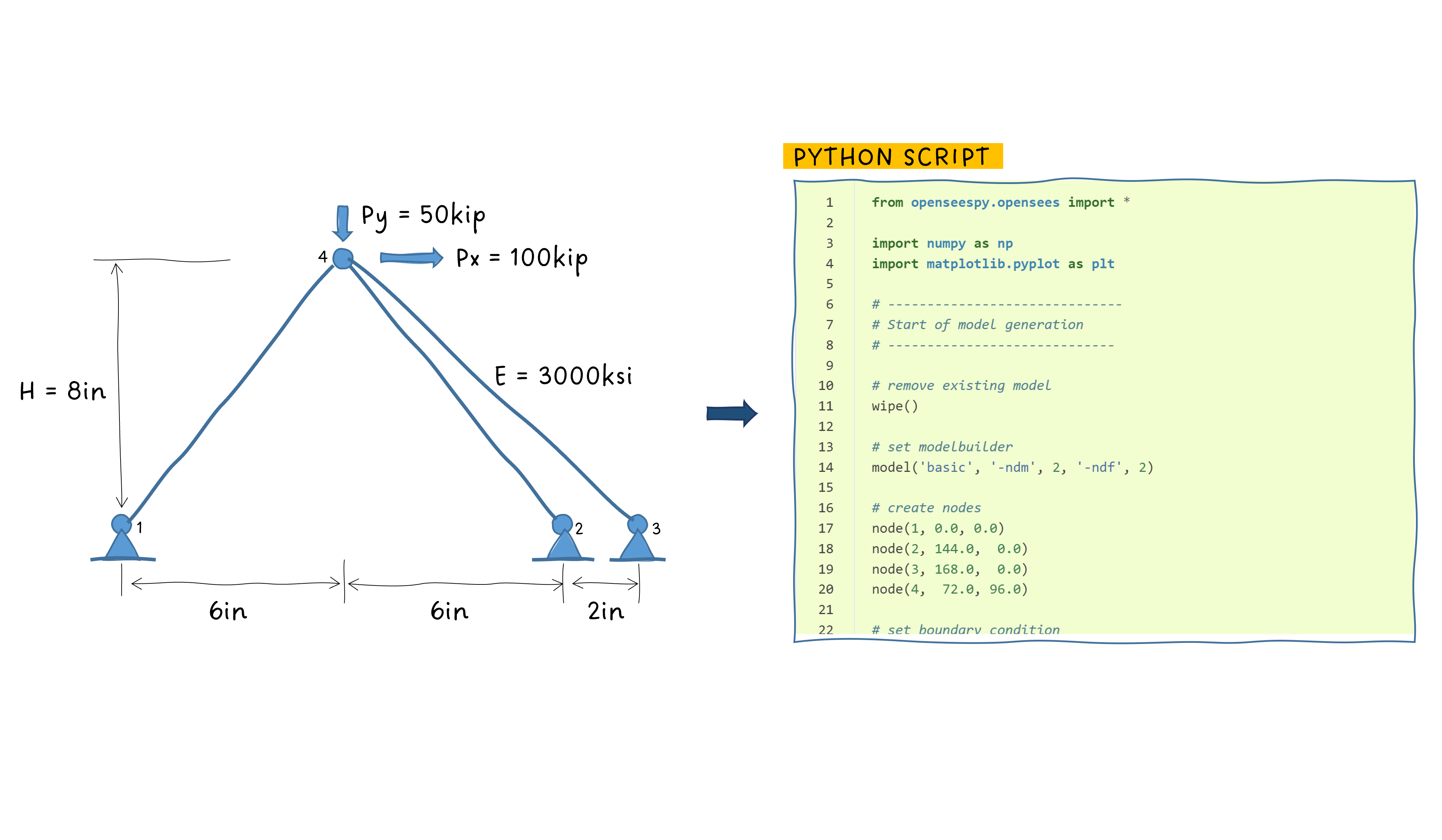
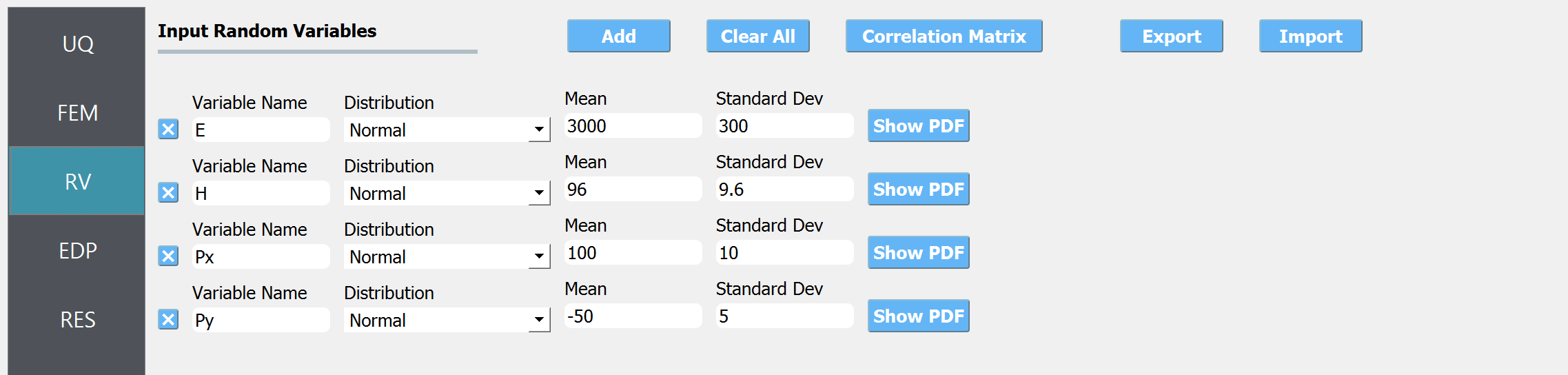
We now need to indicate quoFEM what are the input random variables (RVs) and output Quantities of Interest (QoIs). Let us consider the following setup:

Four RVs: height ($H$), elastic modulus ($E$), horizontal load ($P_x$), vertical load ($P_y$)
Two QoIs: horizontal and vertical displacements of node 4 ($u_x$ and $u_y$)

To convey this information to quoFEM, the following steps are needed.

Create a parameter file, params.py, that contains the below four lines, in the folder TrussExample:

E = 3000.0 # elastic modulus
H = 96.0 # height
Px = 100.0 # xForce
Py = -50.0 # yForce
This indicates quoFEM the list RVs

Note

The specified values are not actually used in the quoFEM analysis, because they will be overwritten according to the probability distribution specified in Step 2.

Modify the main script ElasticTruss.py as follows (the modified parts are highlighted in the code)
- Import params.py on top of the main script
- Replace the hard-coded values of RVs with the variables H, E, Px, and Py
- Write QoI values (ux and uy) to results.out

from openseespy.opensees import *

import numpy as np
import matplotlib.pyplot as plt
from params import *
# ------------------------------
# Start of model generation
# -----------------------------

# remove existing model
wipe()

# set modelbuilder
model('basic', '-ndm', 2, '-ndf', 2)

# create nodes
node(1, 0.0, 0.0)
node(2, 144.0,  0.0)
node(3, 168.0,  0.0)
node(4,  72.0,  H)

# set boundary condition
fix(1, 1, 1)
fix(2, 1, 1)
fix(3, 1, 1)

# define materials
uniaxialMaterial("Elastic", 1, E)

# define elements
element("Truss",1,1,4,10.0,1)
element("Truss",2,2,4,5.0,1)
element("Truss",3,3,4,5.0,1)

# create TimeSeries
timeSeries("Linear", 1)

# create a plain load pattern
pattern("Plain", 1, 1)

# Create the nodal load - command: load nodeID xForce yForce
load(4, Px, Py)

# ------------------------------
# Start of analysis generation
# ------------------------------

# create SOE
system("BandSPD")

# create DOF number
numberer("RCM")

# create constraint handler
constraints("Plain")

# create integrator
integrator("LoadControl", 1.0)

# create algorithm
algorithm("Linear")

# create analysis object
analysis("Static")

# perform the analysis
analyze(1)

ux = nodeDisp(4,1)
uy = nodeDisp(4,2)
if abs(ux-0.53009277713228375450)<1e-12 and abs(uy+0.17789363846931768864)<1e-12:
    print("Passed!")
else:
    print("Failed!")

with open("results.out", "w") as f:
        f.write("{} {}".format(ux,uy))             

from openseespy.opensees import *

import numpy as np
import matplotlib.pyplot as plt

# ------------------------------
# Start of model generation
# -----------------------------

# remove existing model
wipe()

# set modelbuilder
model('basic', '-ndm', 2, '-ndf', 2)

# create nodes
node(1, 0.0, 0.0)
node(2, 144.0,  0.0)
node(3, 168.0,  0.0)
node(4,  72.0, 96.0)

# set boundary condition
fix(1, 1, 1)
fix(2, 1, 1)
fix(3, 1, 1)

# define materials
uniaxialMaterial("Elastic", 1, 3000.0)

# define elements
element("Truss",1,1,4,10.0,1)
element("Truss",2,2,4,5.0,1)
element("Truss",3,3,4,5.0,1)

# create TimeSeries
timeSeries("Linear", 1)

# create a plain load pattern
pattern("Plain", 1, 1)

# Create the nodal load - command: load nodeID xForce yForce
load(4, 100.0, -50.0)

# ------------------------------
# Start of analysis generation
# ------------------------------

# create SOE
system("BandSPD")

# create DOF number
numberer("RCM")

# create constraint handler
constraints("Plain")

# create integrator
integrator("LoadControl", 1.0)

# create algorithm
algorithm("Linear")

# create analysis object
analysis("Static")

# perform the analysis
analyze(1)

ux = nodeDisp(4,1)
uy = nodeDisp(4,2)
if abs(ux-0.53009277713228375450)<1e-12 and abs(uy+0.17789363846931768864)<1e-12:
    print("Passed!")
else:
    print("Failed!")

Test Your Model Test your new Python script using the same command used in Step 0.
{$PathToPythonExe} ElasticTruss.py

This time, results.out should be created in the folder TrussExample, which contains the following two values.

Fig. 2.2.4 Created results.out¶

If the test was successful, remove all the files except ElasticTruss.py and params.py. This model can now be readily imported into quoFEM.

Important

It is important to remove results.out file after testing.

Step 2

Step 2. Run quoFEM

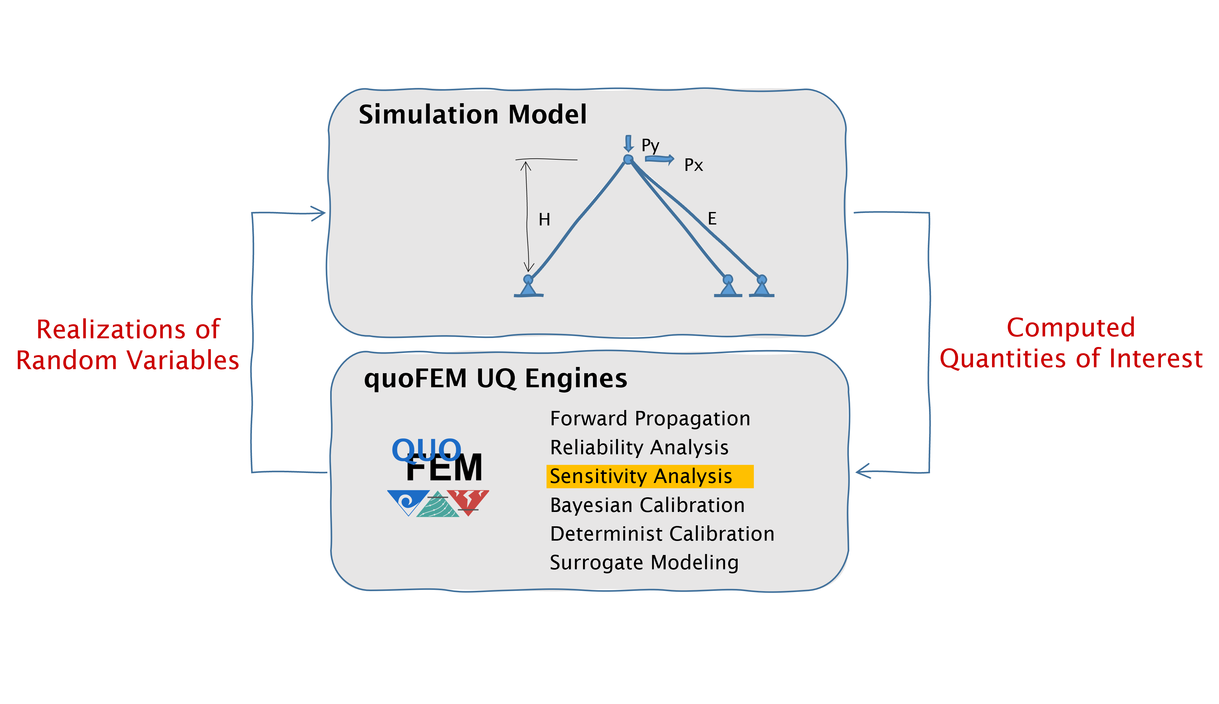
quoFEM has four input taps - UQ, FEM, RV, EDP(QoI)- that guide users to provide the required inputs for the UQ analysis

UQ (Uncertainty Quantification)

We will use dakota-Sensitivity Analysis for this example.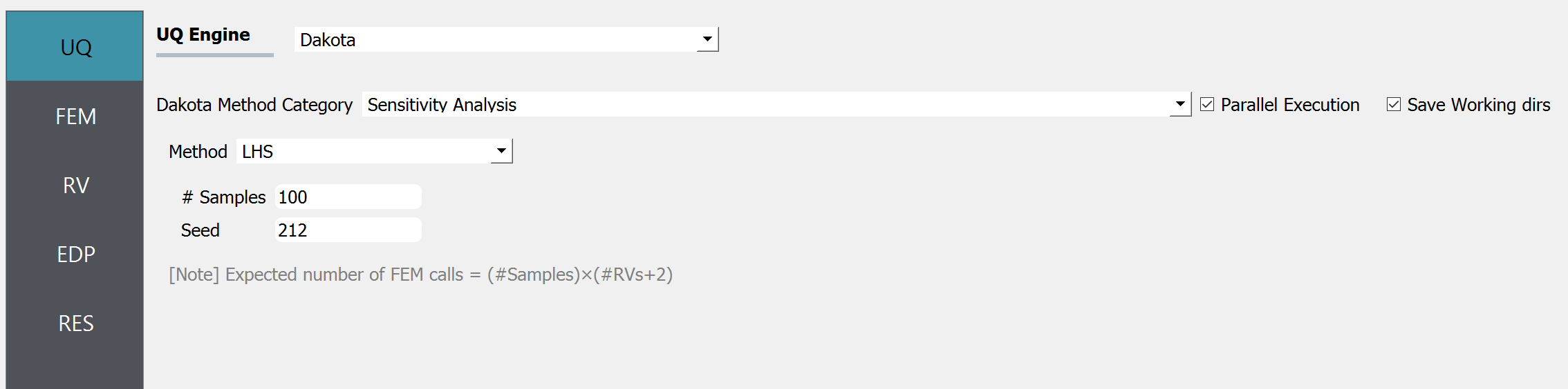

Fig. 2.2.5 UQ Panel¶

Tip

Once the user prepares the input script according to Step 1, they can use it for any UQ analysis supported in quoFEM without additional modifications.

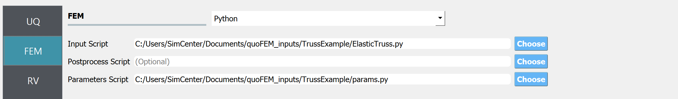
FEM (Finite Element Model or any simulation model)

Import the two model scripts prepared in Step 1 here.

Fig. 2.2.6 FEM Panel¶

The post-processing script is not needed in this example because the results.out is already printed in the main script. See here for more about the post-processing script

RV (Random Variables)

Reading params.py, quoFEM auto-populates the RVs as follows.

Fig. 2.2.7 RV Panel¶

Then one can modify their distribution types and parameters. Further, if you believe some variables are correlated, use the correlation button to specify the values.

Fig. 2.2.8 Correlation Window¶

EDP (Engineering Demand Parameters) or QoI (Quantities of Interest)

Because our Python script will write two values in results.out file, we will specify two QoI as follows.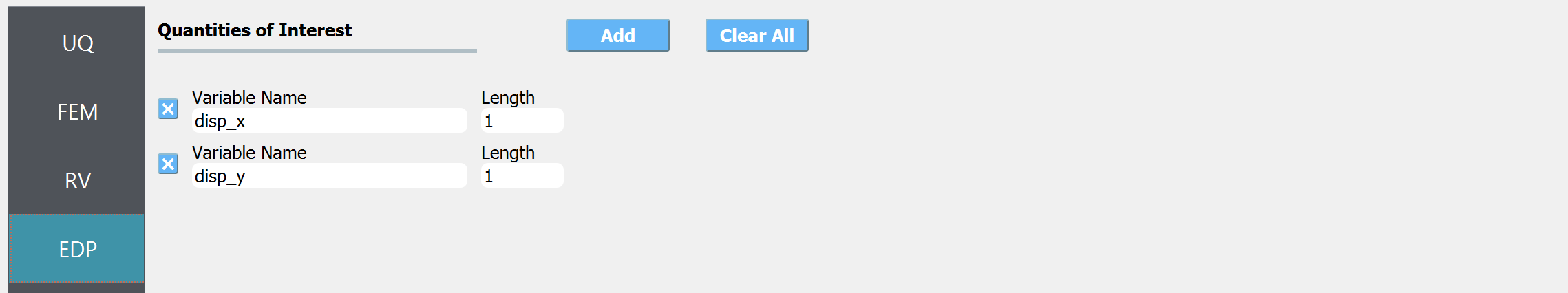

Fig. 2.2.9 EDP Panel¶

The order should match that written in the results.out file, and the specified name of QoIs is used only for the display in this example. Please see here to learn about vector QoIs that have a length greater than 1

When all the fields are filled in, click the Run button, and the analysis will be performed. Do not press the Run button twice - it will give you an error. You can check the progress status in your Local Working directory which can be found in the preference window. The number attached to ‘workdir’. indicates the simulation index, and each folder contains the details for each simulation run.

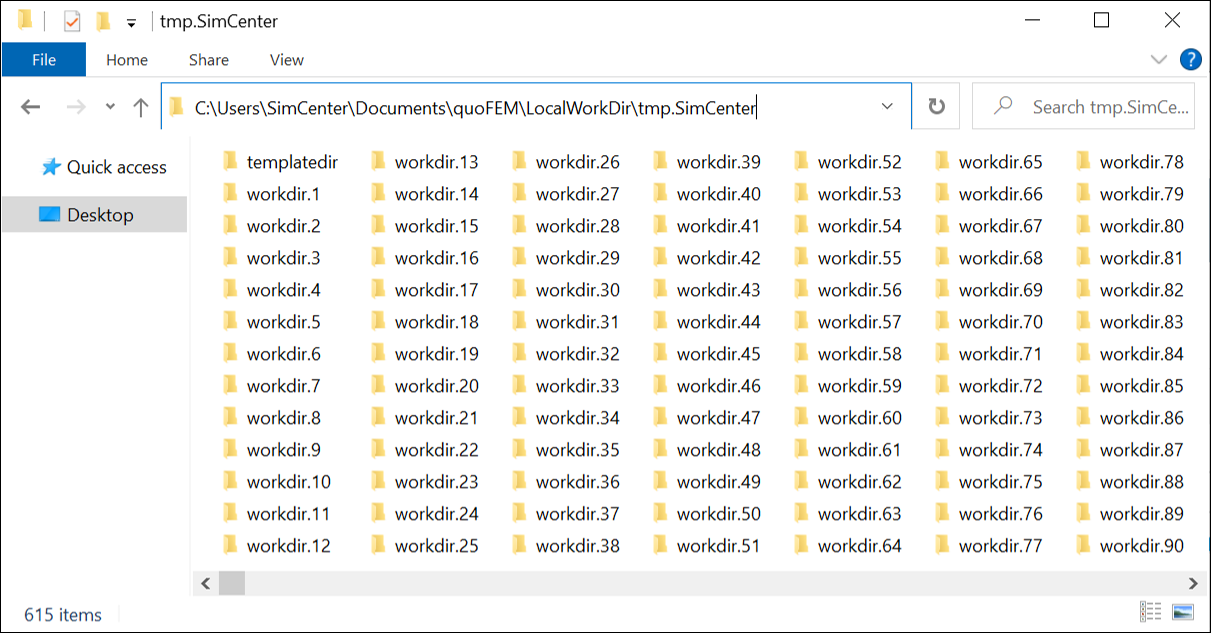
Fig. 2.2.10 Working directories¶

Once the analysis is done, move on to the RES tab.

RES (Results)

The results indicate that the horizontal displacement is most affected by the height while vertical displacement is dominated by the elastic modulus and vertical force.

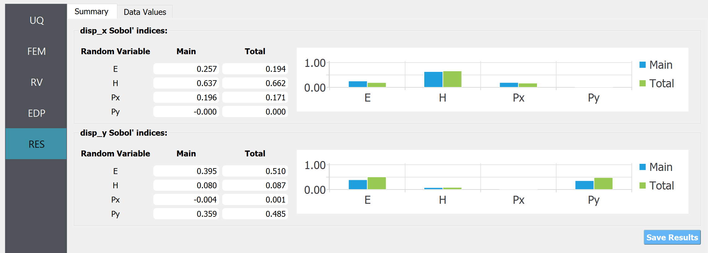
Fig. 2.2.11 RES - Summary¶

And this can be confirmed by the strong/weak trends observed in the scatter plots.

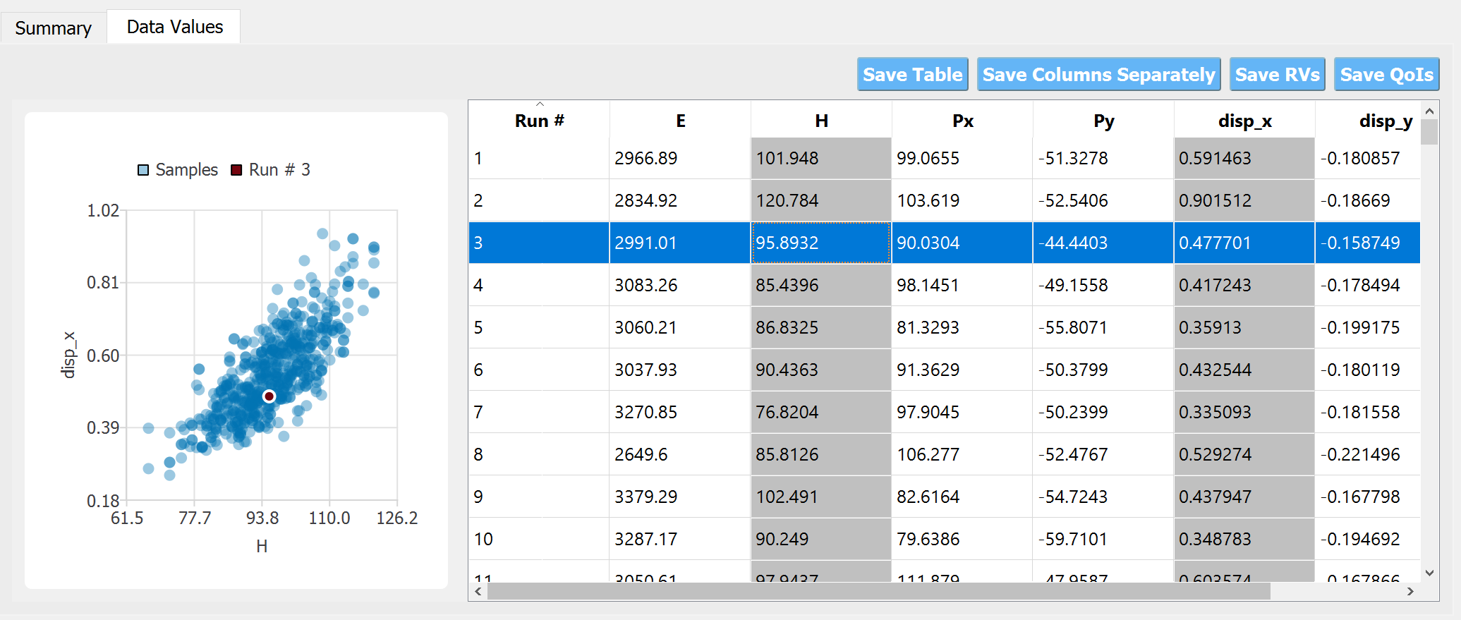
Fig. 2.2.12 RES - Data Values - Scatter plot of H and disp_x¶

The right/left mouse buttons (fn-clink, option-click, or command-click replaces the left click on Mac) will allow the users to draw various scatter plots, histograms, and cumulative mass plots from the sample points.

See Dakota or SimCenterUQ theory manual to learn more about the sensitivity analysis and the difference between main and total indices.

Tip

The global sensitivity analysis results will be different when probability distribution changes (i.e. when the amount of uncertainty in each input variable changes), and users can test different conditions simply by changing the distributions in the RV tab.

Step 3

Step 3. Run quoFEM at DesignSafe

Users can run the same analysis using the high-performance computer at DesignSafe at Texas Super Computing Center (TACC). For this, login to DesignSafe by clicking Login on the right upper corner of quoFEM, or by clicking RUN at DesignSafe Button

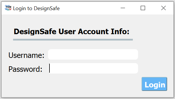
Fig. 2.2.13 Login window¶

If you don’t have a DesignSafe account, you can easily sign up at DesignSafe.

Then by clicking RUN at DesignSafe, one can specify the job details. Please see here for more details on the number of nodes and processors.

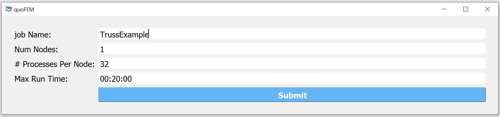
Fig. 2.2.14 Run at DesignSafe¶

If one sets 32 processors, quoFEM will run 32 model evaluations simultaneously in parallel. By clicking Submit, the jobs will be automatically submitted to DesignSafe. (See here to learn more about “What happens when RUN at DesignSafe button is clicked”). Depending on how busy the Frontera at TACC is, your job may start within 30 sec or it may take longer. By clicking GET from DesignSafe, one can check the status. The major stages are Queued, Running, and Finished.

Fig. 2.2.15 Run at DesignSafe¶

Once the status is changed to Finished, select the job name and click Retrieve Data. The quoFEM will load the data. The results should be the same as the local analysis results.

Fig. 2.2.16 Sensitivity Analysis Results from DesignSafe¶

The created results files can be found in your Remote working directory which can be found in the preference window. Furthermore, one can access all the output files and logs created by quoFEM by signing in to DesignSafe and navigating in the menu bar to Workspace - Tools & Applications - Jobs Status (at the right-hand side edge), and clicking More info and View button (See below figures).

Fig. 2.2.17 DesignSafe - Job status¶

Fig. 2.2.18 DesignSafe - See results files¶

Moving forward..

Things to Consider

Installing additional Python packages

On Windows, it is important to install Python packages to the correct Python executable. Please read here about pip-installing Python packages and changing the Python version.

Note

When running at DesignSafe (e.g. Step 3), SimCenter workflow uses its own Python executable installed on the cloud computer. Currently, the only supported Python packages are those installed through the ‘nheri_simcenter’ package. The available list of packages includes - numpy, scipy, sklearn, pandas, tables, pydoe, gpy, emukit, plotly, matplotlib. If your model uses a package beyond this list, quoFEM analysis will fail.

An option to allow user-defined Python packages on DesignSafe is under implementation. Meanwhile, if you need to request to use additional Python packages, please contact us through user forum.

When your model consists of more than one script

You can import only one main Python file in the FEM tab and put all (and only) the files required to run the analysis in the same folder. quoFEM will automatically copy all the files/subfolders in the same directory of the main input script to the working directory.

Debugging

When quoFEM analysis fails and the error message points you to a working directory, often the detailed error messages are written in ops.out file in the directory. Other .log and .err files can have information to help you identify the cause of the failure. Please feel free to ask us through user forum.
When “RUN at DesignSafe” fails
When the remote analysis fails while the local analysis is successful, there can be many reasons. Some of the common cases are Python compatibility issues and missing Python packages, as discussed earlier on this page. Another common cause is related to cross-platform compatibility (Windows/mac versus Linux). This is usually observed in the relative file paths. For example, the below works on Mac and Windows,
getDisp=pd.read_csv(r'TestResult\disp.out', delimiter= ' ')
but will throw an error on Linux. Below will also work on Linux.
getDisp=pd.read_csv(os.path.join('TestResult', "disp.out"), delimiter= ' ')
Questions, bug reports, and feature requests

We have an active user forum, for any users who have questions or feature requests. The response is mostly within 24 hours and usually much less.