Ground Motion Intensity Spatial Correlation Model Options

The regional seismic risk analysis requires the prediction of ground motion intensities at multiple sites. Such joint predictions need to consider the correlation between ground motion intensities at different sites given a specific earthquake scenario. In general, ground motion models predict intensities at an individual site \(i\) due to an earthquake \(j\) have the following form:

()\[ln(Y_{ij}) = ln(\bar{Y}_{ij}) + \epsilon_{ij} + \eta_j\]

where \(Y_{ij}\) is the intensity measure (e.g., \(Sa(T)\)), \(\bar{Y}_{ij}\) is the predicted median intensity (given magnitude, distance, period, and site conditions), \(\epsilon_{ij}\) is the intra-event residual, and \(\eta_j\) is the inter-event residual. It is assumed that \(\epsilon_{ij}\) and \(\eta_j\) are random variables with zero means and standard deviations \(\sigma_{ij}\) and \(\tau_j\).

Note

1. Intra-event residual quantifies the deviation of intensities at different sites given a specific earthquake realization.

2. Inter-event residual quantifies the deviation of intensities at a specific site given different earthquake realizations.

Intra-event Correlation Model Options

[Jayaram08] found that the spatially distributed intra-event residuals \(\epsilon_j = (\epsilon_{1j}, \epsilon_{2j}, ..., \epsilon_{dj})\) follows a multivariate normal distribution. This multivariate normal distribution can be defined by the mean, variance, and correlation (between \(\epsilon_{i_1j}\) and \(\epsilon_{i_2j}\)). The mean is zero (as discussed previously) and the variance can be predicted by ground motion models, but the correlation between residuals at two different sites needs to be described. The semivariogram \(\gamma(u,u^\prime)\) is used to describe the expected squared difference between two locations \(u\) and \(u^\prime\). Because it is very difficult to obtain several observations of a random variable at a given pair of sites, the stationarity assumption is usually applied to simplify it to a more trackable problem. It is typically assumed that the semivariogram only depends on the distance \(h\) - the stationary semivariogram \(\gamma(h)\) can be obtained from data as follows:

()\[\gamma(h) = \frac{1}{2}[E(Z_u - Z_{u+h})^2]\]

where \(Z_u\) and \(Z_{u+h}\) are the random variable realizations at sites with a distance of \(h\). The covariance between \(Z_u\) and \(Z_{u+h}\) are:

()\[C(h) = E[(Z_u - \mu_Z)(Z_{u+h} - \mu_Z)]\]

where \(\mu_Z\) is the mean (which is zero under the stationarity assumption). Note this spatial covariance can also be related to the semivariogram with:

()\[C(h) = C(0) - \gamma(h)\]

Similarly, the correlation coefficient is defined as:

()\[\rho(h) = \frac{C(h)}{C(0)} = 1 - \frac{\gamma(h)}{C(0)}\]

Given the semivariogram is often preferred in geostatistical practice (because it does not require a prior estimation of the mean), many studies were carried to find the semivariogram models to derive the correlation \(rho(h)\) of ground motion intensities. The available models in the current quoFEM app are briefly summarized in following sections.

Jayaram and Baker (2009)

[Jayaram09] adopted a exponential model for the semivariogram function with a isotropic hypothesis (i.e., the distance \(h\) is the separation length):

()\[\gamma(h) = a[1 - exp(-3h / b)]\]

where a and b are two modeling coefficients, namely sill and the range of the semivariogram function, respectively. When \(h = 0\), \(\gamma(h=0) = 0\) which leads to \(\rho(h = 0) = 1\). As the distance between two sites increases, i.e., \(h\) increases, \(\gamma(h)\) increases and \(\rho(h)\) decreases, which is consistent with the decaying trend of correlation between the two sites. After calibrating the model to past earthquake recordings, the following model was proposed for predicting the spatial correlation \(\rho(h)\):

()\[\rho(h) = exp(-3h / b)\]

The range of the semivariogram function \(b\) was found to depend on the similarity of \(V_{S30}\) values in the given region. If the \(V_{S30}\) values do not show clustering, the \(b\) is computed by:

()\[ \begin{align}\begin{aligned}b = 8.5 + 17.2T, T < 1s\\b = 22.0 + 3.7T, T \leq 1s\end{aligned}\end{align} \]

where T is the period. If the \(V_{S30}\) values are very close in the given region, the \(b\) can be computed by:

()\[ \begin{align}\begin{aligned}b = 40.7 - 15.0T, T < 1s\\b = 22.0 + 3.7T, T \leq 1s\end{aligned}\end{align} \]

Note

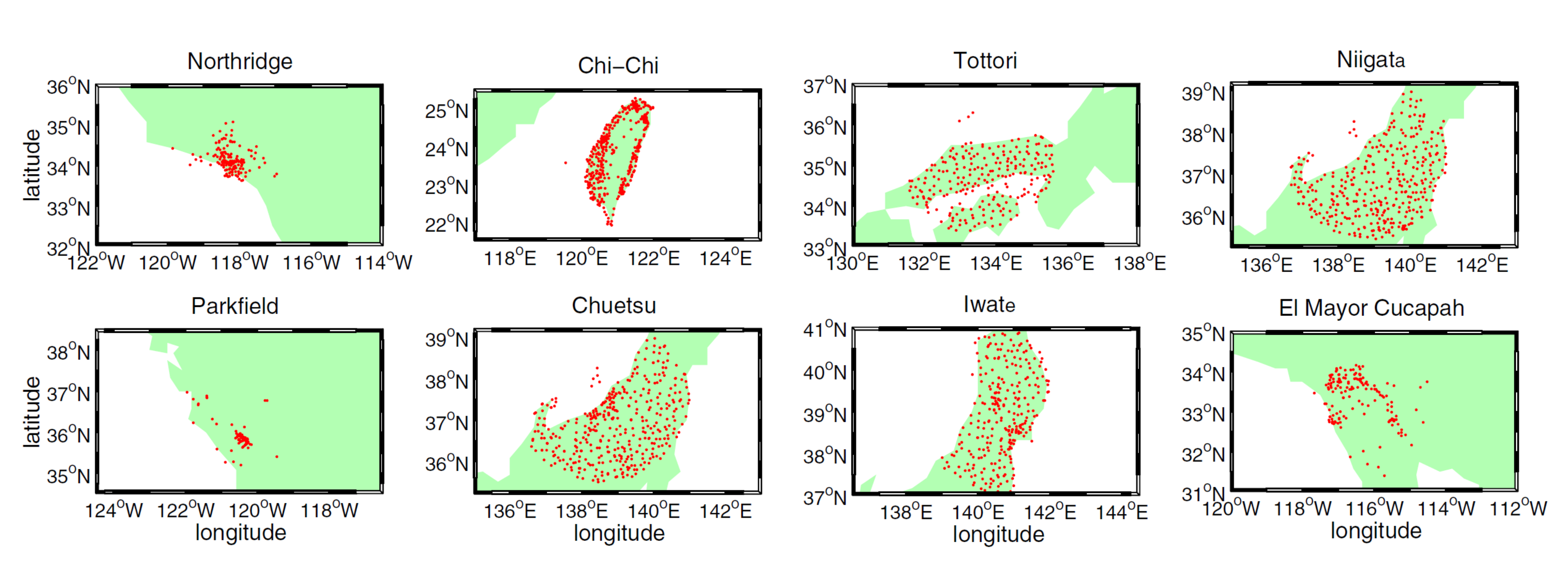
Earthquakes that were considered in the development: Anza earthquake, Alum Rock earthquake, Parkfield earthquake, Chi-Chi earthquake, Northridge earthquake, Big Bear City earthquake, and Chino Hills earthquake.

Loth and Baker (2013)

Note that the cross-semivariograms between different pairs of intensity measures can be different, for instance, \(\rho_{Sa(T=0.1s),Sa(T=0.2s)}(h)\) might be greater than \(\rho_{Sa(T=0.1s),Sa(T=1s)}(h)\). This means one needs to repeat a calibration process many times to develop semivariogram functions and correlation models that have higher resolutions (i.e., direct semivariogram fit). Instead of fitting each semivariogram independently, [Loth13] proposed a predictive model for spatial covariance of spectral accelerations at different periods:

()\[\textbf{C}(h) = \textbf{B}^1 exp(-3h/20) + \textbf{B}^2 exp(-3h/70) + \textbf{B}^3 I_{h=0}\]

where \(I_{h=0}\) is the indicator function equal to 1 at \(h = 0\) and 0 otherwise. And the three coefficient matrices \(\textbf{B}^1\), \(\textbf{B}^2\), and \(\textbf{B}^3\) were calibrated by 2080 recordings from 8 earthquakes.

Location of recordings from the 8 earthquakes considered by [Loth13]

Short-range coregionalization matrix, \(\textbf{B}^1\)

Periods (s)	0.01	0.1	0.2	0.5	1.0	2.0	5.0	7.5	10.0
0.01	0.29	0.25	0.23	0.23	0.18	0.10	0.06	0.06	0.06
0.1	0.25	0.30	0.20	0.16	0.10	0.04	0.03	0.04	0.05
0.2	0.23	0.20	0.27	0.18	0.10	0.03	0.00	0.01	0.02
0.5	0.23	0.16	0.18	0.31	0.22	0.14	0.08	0.07	0.07
1.0	0.18	0.10	0.10	0.22	0.33	0.24	0.16	0.13	0.12
2.0	0.10	0.04	0.03	0.14	0.24	0.33	0.26	0.21	0.19
5.0	0.06	0.03	0.00	0.08	0.16	0.26	0.37	0.30	0.26
7.5	0.06	0.04	0.01	0.07	0.13	0.21	0.30	0.28	0.24
10.0	0.06	0.05	0.02	0.07	0.12	0.19	0.26	0.24	0.23

Short-range coregionalization matrix, \(\textbf{B}^2\)

Periods (s)	0.01	0.1	0.2	0.5	1.0	2.0	5.0	7.5	10.0
0.01	0.47	0.40	0.43	0.35	0.27	0.15	0.13	0.09	0.12
0.1	0.40	0.42	0.37	0.25	0.15	0.03	0.04	0.00	0.03
0.2	0.43	0.37	0.45	0.36	0.26	0.15	0.09	0.05	0.08
0.5	0.35	0.25	0.36	0.42	0.37	0.29	0.20	0.16	0.16
1.0	0.27	0.15	0.26	0.37	0.48	0.41	0.26	0.21	0.21
2.0	0.15	0.03	0.15	0.29	0.41	0.55	0.37	0.33	0.32
5.0	0.13	0.04	0.09	0.20	0.26	0.37	0.51	0.49	0.49
7.5	0.09	0.00	0.05	0.16	0.21	0.33	0.49	0.62	0.60
10.0	0.12	0.03	0.08	0.16	0.21	0.32	0.49	0.60	0.68

Short-range coregionalization matrix, \(\textbf{B}^3\)

Periods (s)	0.01	0.1	0.2	0.5	1.0	2.0	5.0	7.5	10.0
0.01	0.24	0.22	0.21	0.09	-0.02	0.01	0.03	0.02	0.01
0.1	0.22	0.28	0.20	0.04	-0.05	0.00	0.01	0.01	-0.01
0.2	0.21	0.20	0.28	0.05	-0.06	0.00	0.04	0.03	0.01
0.5	0.09	0.04	0.05	0.26	0.14	0.05	0.05	0.04	0.04
1.0	-0.02	-0.05	-0.06	0.14	0.20	0.07	0.05	0.05	0.05
2.0	0.01	0.00	0.00	0.05	0.07	0.12	0.08	0.07	0.06
5.0	0.03	0.01	0.04	0.05	0.05	0.08	0.12	0.10	0.08
7.5	0.02	0.01	0.03	0.05	0.05	0.07	0.10	0.10	0.09
10.0	0.01	-0.01	0.01	0.04	0.05	0.06	0.08	0.09	0.09

Markhvida et al. (2017)

[Markhvida17] proposed to use Principal Component Analysis (PCA) to develop the predictive model for cross-correlograms. In theorem, PCA performs a linear transformation of the variables of interests to an orthogonal basis, where the resulting projections onto the new basis are uncorrelated:

()\[\textbf{P} \textbf{Z} = \textbf{Y}\]

where \(\textbf{P}\) is an orthogonal linear transformation matrix, \(\textbf{Z}\) is the original data matrix, and \(\textbf{Y}\) is the transformed variable matrix which contains uncorrelated principal components \(\textbf{Y}_i\). Since \(\textbf{P}\) is orthogonal, so the inversion is easy to compute:

()\[\textbf{Z} = \textbf{P}^{-1} \textbf{Y} = \textbf{P}^{T} \textbf{Y}\]

For each principal component, one covariance model is developed:

()\[C_i(h) = c_{0i}I_{h=0} + c_{1i} exp(-3h/a_{1i}) + c_{2i} exp(-3h/a_{2i})\]

where \(c_{0i}\), \(c_{1i}\), \(c_{2i}\), \(a_{1i}\), and \(a_{2i}\) are modeling coefficients for \(i^{th}\) principal component. Instead of directly simulating the desired intensity measures, this PCA-based method would first simulate uncorrelated variables using \(C_i(h)\) and then transform them back to intensity measures.

Principal component transformation coefficients

Periods (s)	0.01	0.02	0.03	0.05	0.075	0.1	0.15	0.2	0.25	0.3	0.4	0.5	0.75	1.0	1.5	2.0	3.0	4.0	5.0
0.01	0.27	-0.14	0.07	-0.11	-0.09	-0.11	-0.19	0.15	-0.16	-0.05	0.11	0.05	-0.08	0.00	0.23	-0.04	-0.30	-0.53	-0.58
0.02	0.27	-0.14	0.08	-0.12	-0.10	-0.12	-0.20	0.16	-0.16	-0.05	0.10	0.05	-0.08	0.01	0.22	-0.04	-0.26	-0.15	0.78
0.03	0.27	-0.15	0.10	-0.14	-0.13	-0.15	-0.22	0.15	-0.14	-0.05	0.09	0.04	-0.06	0.01	0.15	-0.02	-0.03	0.81	-0.23
0.05	0.25	-0.18	0.18	-0.22	-0.18	-0.18	-0.19	0.04	-0.05	-0.03	-0.03	-0.06	0.09	0.02	-0.30	0.06	0.75	-0.21	0.02
0.075	0.24	-0.22	0.24	-0.23	-0.13	-0.04	0.12	-0.27	0.24	0.10	-0.26	-0.12	0.20	0.01	-0.49	0.12	-0.48	0.04	-0.01
0.1	0.23	-0.23	0.23	-0.16	0.04	0.18	0.43	-0.32	0.26	0.14	-0.08	0.05	-0.15	-0.08	0.53	-0.18	0.21	-0.00	0.00
0.15	0.24	-0.21	0.13	0.08	0.33	0.39	0.33	0.16	-0.18	-0.14	0.47	0.18	-0.11	0.09	-0.29	0.26	-0.00	0.02	0.00
0.2	0.25	-0.17	-0.01	0.28	0.40	0.22	-0.08	0.22	-0.17	-0.03	-0.38	-0.24	0.36	-0.09	-0.01	-0.44	0.02	0.01	0.00
0.25	0.25	-0.12	-0.15	0.37	0.25	-0.06	-0.28	-0.08	0.21	0.14	-0.28	-0.04	-0.20	0.02	0.16	0.63	0.05	0.00	0.00
0.3	0.25	-0.07	-0.24	0.36	0.04	-0.25	-0.14	-0.29	0.30	0.06	0.33	0.21	-0.19	0.03	-0.26	-0.48	0.00	0.01	0.00
0.4	0.25	0.01	-0.33	0.23	-0.26	-0.22	0.34	-0.12	-0.06	-0.22	0.21	-0.13	0.58	-0.06	0.20	0.21	0.02	0.00	0.00
0.5	0.25	0.08	-0.36	0.06	-0.34	0.02	0.39	0.18	-0.26	-0.01	-0.38	-0.08	-0.50	0.02	-0.18	-0.07	0.02	0.01	0.00
0.75	0.23	0.19	-0.34	-0.22	-0.17	0.42	-0.14	0.19	0.15	0.53	0.04	0.33	0.27	0.06	0.00	0.01	0.02	0.00	0.00
1.0	0.21	0.26	-0.24	-0.33	0.08	0.33	-0.22	-0.12	0.27	-0.44	0.15	-0.48	-0.14	-0.04	0.01	-0.02	-0.01	0.00	-0.00
1.5	0.19	0.33	-0.09	-0.27	0.36	-0.15	-0.00	-0.33	-0.27	-0.28	-0.26	0.53	0.07	-0.08	-0.03	0.03	0.01	0.00	-0.00
2.0	0.18	0.36	0.06	-0.16	0.35	-0.34	0.16	-0.03	-0.21	0.51	0.21	-0.41	-0.04	0.17	-0.00	-0.01	-0.01	0.00	0.00
3.0	0.17	0.36	0.26	0.07	0.06	-0.22	0.18	0.52	0.46	-0.10	-0.02	0.12	-0.00	-0.42	-0.04	0.02	0.01	-0.01	0.00
4.0	0.16	0.35	0.35	0.24	-0.16	0.09	-0.01	0.02	0.11	-0.18	-0.12	0.07	0.06	0.75	0.08	-0.05	0.00	-0.00	-0.00
5.0	0.15	0.33	0.37	0.33	-0.28	0.28	-0.18	-0.33	-0.31	0.13	0.08	-0.07	-0.05	-0.44	-0.04	0.03	3.0	0.00	0.00

The general idea is to include more degrees of freedom in the predictive model if compared to linear models (e.g., [Loth13]). The figure below contrasts the correlation coefficient functions by PCA and the linear model by [Loth13].

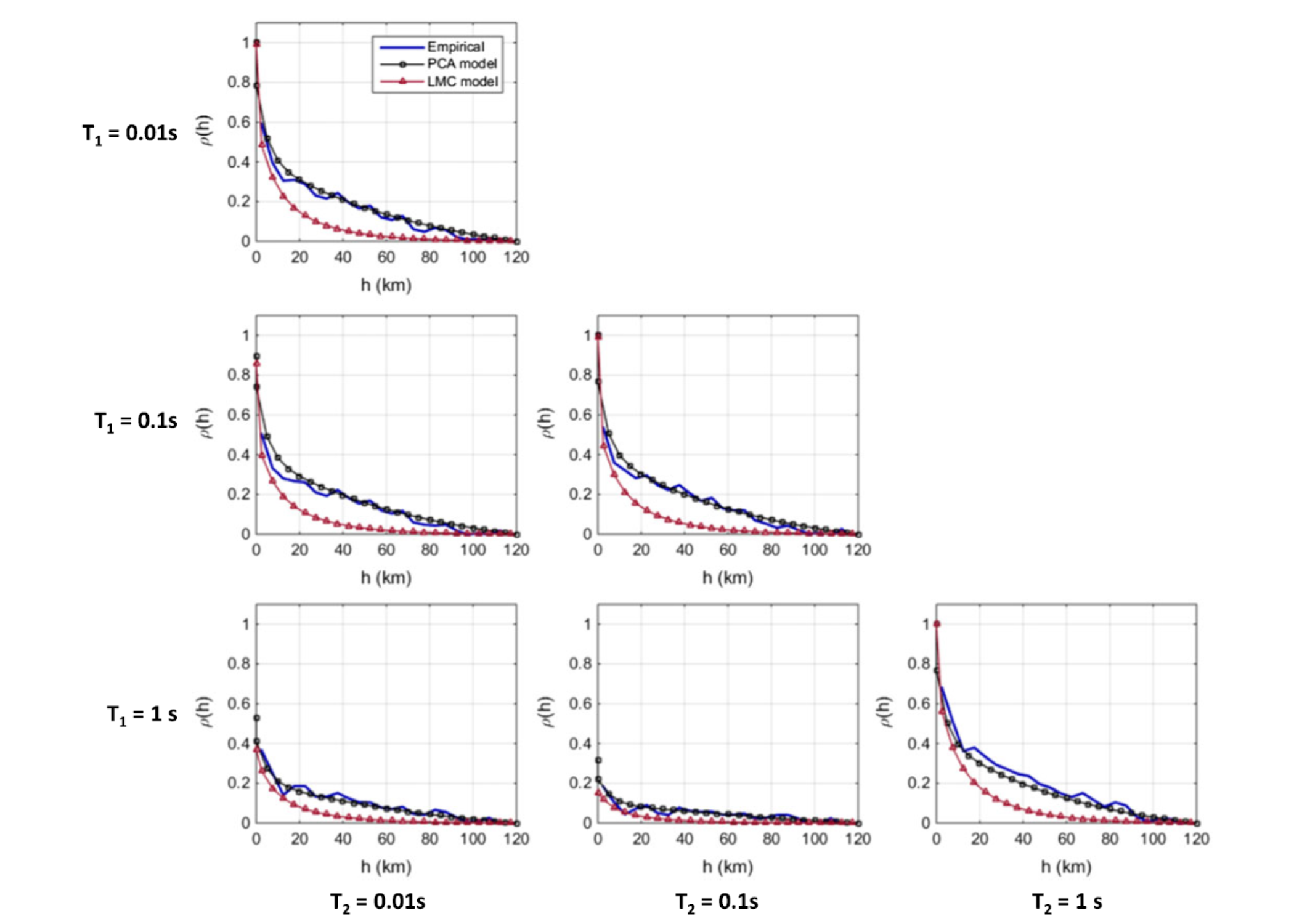
Comparison of principal component analysis (PCA) model and linear model of coregionalization (LMC) correlograms and cross-correlograms ([Loth13]) for different periods

Jayaram08

Jayaram N, Baker JW. Statistical tests of the joint distribution of spectral acceleration values. Bulletin of the Seismological Society of America 2008; 98(5):2231–2243.

Jayaram09

Jayaram, N., & Baker, J. W. (2009). Correlation model for spatially distributed ground‐motion intensities. Earthquake Engineering & Structural Dynamics, 38(15), 1687-1708.

Loth13(1,2,3,4,5)

Loth, C., & Baker, J. W. (2013). A spatial cross‐correlation model of spectral accelerations at multiple periods. Earthquake Engineering & Structural Dynamics, 42(3), 397-417.

Markhvida17

Markhvida, M., Ceferino, L., & Baker, J. W. (2018). Modeling spatially correlated spectral accelerations at multiple periods using principal component analysis and geostatistics. Earthquake Engineering & Structural Dynamics, 47(5), 1107-1123.

Inter-event Correlation Model Options

[Baker08] presented equations to predict the inter-event residual correlations of spectral acceleration values, using the Next Generation Attenuation (NGA) ground motion library and the new NGA ground motion models (GMMs). A predictive equation was presented that provides correlations between logarithmic spectral accelerations at two periods. This equation was observed to be valid for a variety of definitions of spectral acceleration (i.e., spectral acceleration of an individual component, the geometric mean of spectral accelerations from two orthogonal components, and the orientation-independent GMRotI definition used by the NGA modelers)

The correlation equations are applicable for use with any of the NGA ground motion models at periods between 0.01 and 10 seconds. When the periods of interest are less than 5 seconds, correlation coefficients from all considered models are essentially identical. If one period is greater than 5 seconds and the second period is significantly less than 5 seconds, correlations vary slightly among models. These variations are likely due to a lack of empirical data, and these widely-spaced period pairs are also of less engineering interest, so separate correlation equations were not developed for each model. The similarity of correlations from the various GMMs occurs because the correlations are dominated by the large record-to-record variability in observed spectral values from similar events. While slight differences in mean predicted values from the GMMs may be important for some applications, they do not affect computed values to a large enough extent that correlations change noticeably. The predictive equations (Eq. 5 and Eq. 6 in [Baker08]) are implemented in R2D.

Baker08(1,2)

Baker, J. W., & Jayaram, N. (2008). Correlation of spectral acceleration values from NGA ground motion models. Earthquake Spectra, 24(1), 299-317.