4.4. Steel Frame: Conventional Calibration

Problem files

Download

4.4.1. Outline

In this example, a parameter estimation routine is used to estimate column stiffnesses of a simple steel frame, given synthetic data about its mode shapes and frequencies, by minimizing the sum of the squared errors between the data and the model predictions.

4.4.2. Problem description

This example is provided by Professor Joel Conte and his doctoral students Maitreya Kurumbhati and Mukesh Ramancha from UC San Diego.

4.4.2.1. Structural system

Consider the two-story building structure shown in Fig. 4.4.2.1.1. Each floor slab is made of a composite metal deck and is supported on the steel columns. These four columns are fixed at the base. The story height is \(h = 10'\), length of each slab is \(33'4''\) and \(30'\) along the X and Y direction, respectively. \(m_1 = 0.52 kips-s^2/in\) and \(m_2 = 0.26 kips-s^2/in\) are the total mass of floor 1 and floor 2, respectively. For the steel columns, Young’s modulus is \(E_s^{col} = 29000 ksi\) and the moment of inertia \(I_{yy}^{col} = 1190 in^4\).

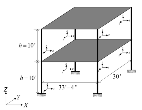
Fig. 4.4.2.1.1 Steel structural system being studied in this example.

4.4.2.2. Finite element model

In this example, only the response of the system along the X direction is considered. For modeling purposes, the floor diaphragms are assumed rigid both in plane and in flexure, and the columns are assumed axially rigid. The structure is modeled as a two-story 2D shear building model as shown in Fig. 4.4.2.2.1. The finite element (FE) software framework OpenSees is utilized for modeling and analysis of the considered structural system. The developed FE model consists of 6 nodes and 6 elastic beam-column elements. To simulate the flexural rigidity of the floors, the moment of inertia \(I_{yy}\) of the horizontal elements is set to a very large number. The horizontal degrees of freedom of node 3 and node 4 are constrained to be equal throughout the analysis to mimic the axial rigidity of floor 1. Similar modeling is performed for floor 2. The vertical displacements of nodes 3, 4, 5, and 6 are constrained to be zero to model the axial rigidity of the columns (see roller supports in Fig. 4.4.2.2.1). After making these modeling assumptions, the only active degrees of freedom of the FE model are the horizontal displacements (translations) of floors 1 and 2, \(u_1\) and \(u_2\), respectively, as shown in Fig. 4.4.2.2.1.

A translational mass \(m_1/2\) and \(m_2/2\) is lumped at the nodes of floor 1 and 2, respectively, along the X direction. The lateral story stiffnesses \(k_1\) and \(k_2\) of story 1 and 2, respectively, are equal to \(48 E_s^{col} I_{yy}^{col}/{h^3}\).

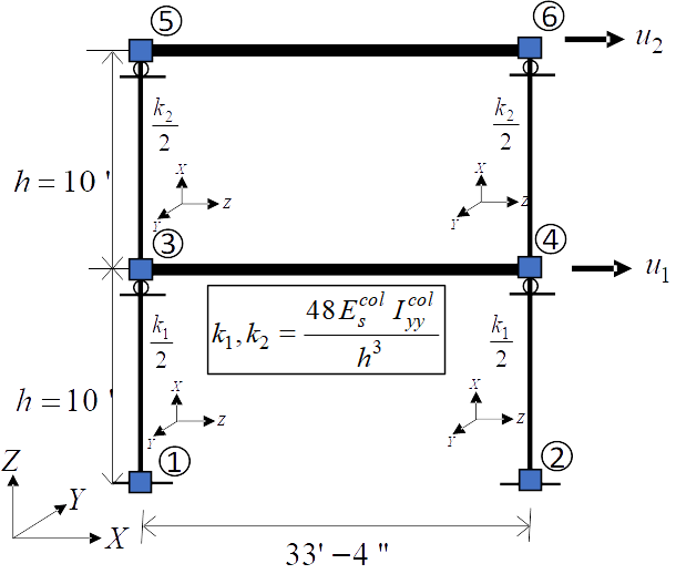
Fig. 4.4.2.2.1 Model of the structural system used in finite element analysis.

4.4.2.3. Natural vibration frequencies and mode shapes

Since the shear building model shown in Fig. 4.4.2.2.1 has only two degrees of freedom, it has two natural modes of vibration. Let \(\lambda_i\) and \(\phi_i\) be the \(i^{th}\) eigenvalue and its corresponding eigenvector, respectively. The two eigenvalues and eigenvectors are obtained by solving the generalized eigenvalue problem of the considered system in OpenSees. The following two eigenvalues are obtained:

(4.4.2.3.1)\[\begin{array}{l} \lambda_1 = 1084.06 (rad/s)^2, \quad \lambda_2 = 6318.34 (rad/s)^2 \end{array}\]

The corresponding eigenvectors (see degrees of freedom u1 and u2 in Fig. 4.4.2.2.1) are given by:

(4.4.2.3.2)\[\begin{split}\phi_1 = \begin{pmatrix}\phi_{11} \\ \phi_{12}\end{pmatrix} = \begin{pmatrix}1.00 \\ 1.41\end{pmatrix} in, \qquad \phi_2 = \begin{pmatrix}\phi_{21} \\ \phi_{22}\end{pmatrix} = \begin{pmatrix}1.00 \\ -1.41\end{pmatrix} in\end{split}\]

The eigenvectors in (4.4.2.3.2) are normalized such that the first component is 1.0. The two vibration mode shapes are shown in Fig. 4.4.2.3.1.

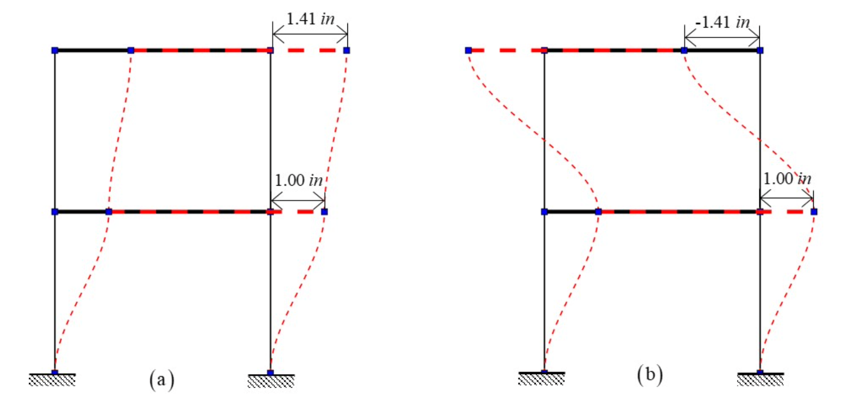
Fig. 4.4.2.3.1 Natural vibration mode shapes: (a) Mode 1 (b) Mode 2.

4.4.2.4. Parameters to be estimated

The FE model of a real structural system often consists of parameters that are unknown to some degree. For example, the parameters related to the mass or stiffness or damping of the system might be unknown. The goal of parameter estimation is to estimate such unknown parameters using some measurement data. The measurement data is obtained by using sensors deployed on the real system. To demonstrate the parameter estimation concept/framework on the considered two-story building system, the first and second story column moment of inertias, \(I_{c1}\) and \(I_{c2}\), are assumed to be unknown while the mass parameters are assumed to be known. In this illustration example, the unknown parameter vector \(\mathbf{\theta}=(I_{c1}, I_{c2})^T\) is estimated using the first eigenvalue and the first eigenvector data.

4.4.2.5. Synthetic data generation

In a real-world application, data on the first eigenvalue and the first eigenvector would consist of system identification results obtained from sensor measurement data. Note that the considered two-story building structure (see Fig. 4.4.2.1.1) is used here as a conceptual/pedagogical example and does not exist in the real world. Therefore, sensor measurement data cannot be collected from the system. As a substitute, measurement data (in the form of estimated first eigenvalue and first eigenvector) are artificially simulated for the purpose of this example, i.e., system identification results for \(\lambda_i\) and \(\phi_i\) from multiple ambient vibration datasets are simulated. To simulate these system identification results (i.e., measurement data), an eigenvalue analysis of the system is performed assuming the following true principal moment of inertia of the columns:

(4.4.2.5.1)\[\mathbf{\theta}^{true} = \left(I_{c1}^{true}, I_{c2}^{true}\right)^T; \quad I_{c1}^{true} = I_{c2}^{true} = 1190 in^4.\]

The corresponding first eigenvalue and first eigenvector are:

(4.4.2.5.2)\[\mathbf{y}^{true} = \left(\lambda_1^{true} = 1084.06 (rad/s)^2, \phi_{12}^{true} = 1.41 in\right)^T\]

To simulate system identification results (measurement data), random estimation errors are added to \(\lambda_1^{true}\) and \(\phi_{12}^{true}\). The random estimation errors for \(\lambda_1^{true}\) and \(\phi_{12}^{true}\) are assumed to be statistically independent, zero-mean Gaussian with 5% coefficient of variation (relative to \(\lambda_1^{true}\) and \(\phi_{12}^{true}\)). Thus, the standard deviation of the system identification errors for \(\lambda_1^{true}\) and \(\phi_{12}^{true}\) are

(4.4.2.5.3)\[\sigma_{\lambda_1}^{true} = 0.05*\lambda_1^{true} = 54.203; \quad \sigma_{\phi_{12}}^{true} = 0.05*\phi_{12}^{true} = 0.0705\]

Now five independent sets of system identification results (measurement data sets) are simulated as:

(4.4.2.5.4)\[\begin{split}\begin{array}{l} \lambda_{1}^{(1)}=1025.21, \quad \lambda_{1}^{(2)}=1138.11, \quad \lambda_{1}^{(3)}=1099.39, \quad \lambda_{1}^{(4)}=1002.41, \quad \lambda_{1}^{(5)}=1052.69 \\ \phi_{12}^{(1)}=1.53, \quad \phi_{12}^{(2)}=1.24, \quad \phi_{12}^{(3)}=1.38, \quad \phi_{12}^{(4)}=1.50, \quad \phi_{12}^{(5)}=1.35 \end{array}\end{split}\]

4.4.2.6. Parameter estimation setup

Our goal will be to estimate the column moments of inertia from the data in (4.4.2.5.4) using a conventional calibration procedure (i.e., a method based on non-linear least squares minimization of the sum of the squared errors between the data and the model predictions).

The unknown quantities of interest are the moments of inertia for the first and second story columns (Ic1 and Ic2 respectively), on which we impose the the following bounds and initial estimates:

1. First story column moment of inertia, Ic1: ContinuousDesign distribution with an initial point \((X_0)\) of \(1500.0\), lower bound \((L_B)\) of \(500.0\), upper bound \((U_B)\) of \(2000.0\),

2. Second story column moment of inertia, Ic2: ContinuousDesign distribution with an initial point \((X_0)\) of \(500.0\), lower bound \((L_B)\) of \(500.0\), upper bound \((U_B)\) of \(2000.0\),

4.4.3. Files required

The exercise requires two files. The user is required to download these file and place them in a new folder.

Warning

Do not place the files in your root, downloads, or desktop folder, as when the application runs it will copy the contents on the directories and subdirectories containing these files multiple times. If you are like us, your root, Downloads or Documents folders contains a lot of files.

The files:

1. fem.tcl - an OpenSees script file that builds the FE model described earlier, conducts an FE analysis, and returns the outputs from the model in a file called results.out.

2. eigData.csv - the calibration data file, which contains the synthetically generated data in five rows and two columns, the contents of which are shown below.

1025.21, 1.53
1138.11, 1.24
1099.39, 1.38 
1002.41, 1.50				
1052.69, 1.35

Note

Since the tcl script creates a results.out file when it runs, no postprocessing script is needed.

4.4.4. UQ workflow

Note

This is the Steel Frame: Deterministic Calibration example in the quoFEM Examples menu. Selecting this example from the menu will autopopulate all the input fields required to run this example. The procedure outlined below demonstrates how to manually set up this problem in quoFEM.

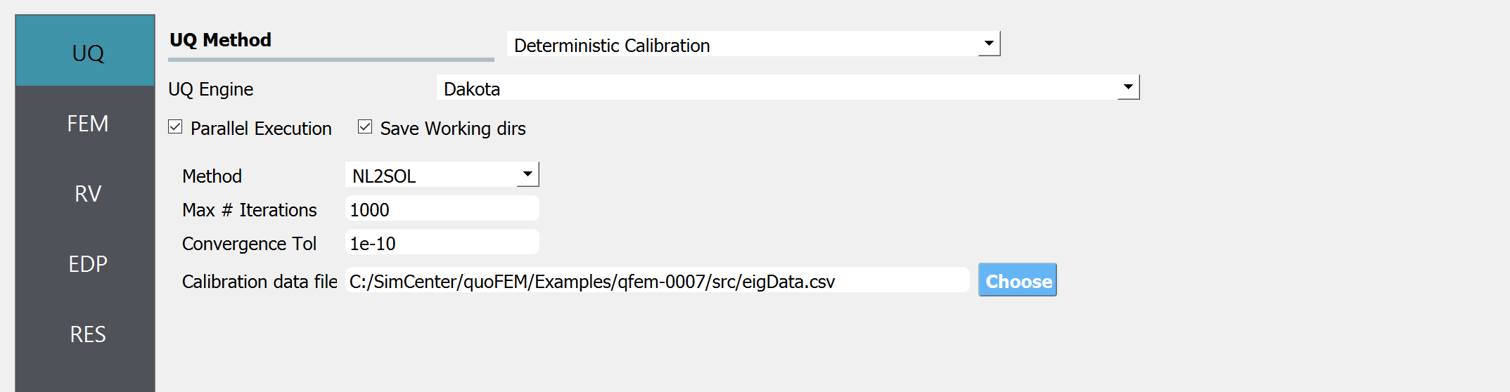
1. Start the application and the UQ panel will be presented. In the panel for the UQ selection, keep the UQ engine as that selected, i.e. Dakota. In the UQ Method category drop down menu change the category to Parameters Estimation, and the method as NL2SOL, and enter the fields as shown in the figure below. If manually setting up this problem, choose the path to the file containing the calibration data on your system.

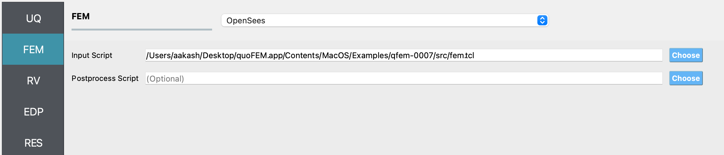
2. Next select the FEM tab from the input panel selection. This will default to the OpenSees FEM engine. For the main script copy the path name to the fem.tcl file or select choose and navigate to the file.

Note

As discussed previously, but worth noting again - since the script generates a results.out file, no postprocessing script is needed for this example. This might not always be the case for some of your problems.

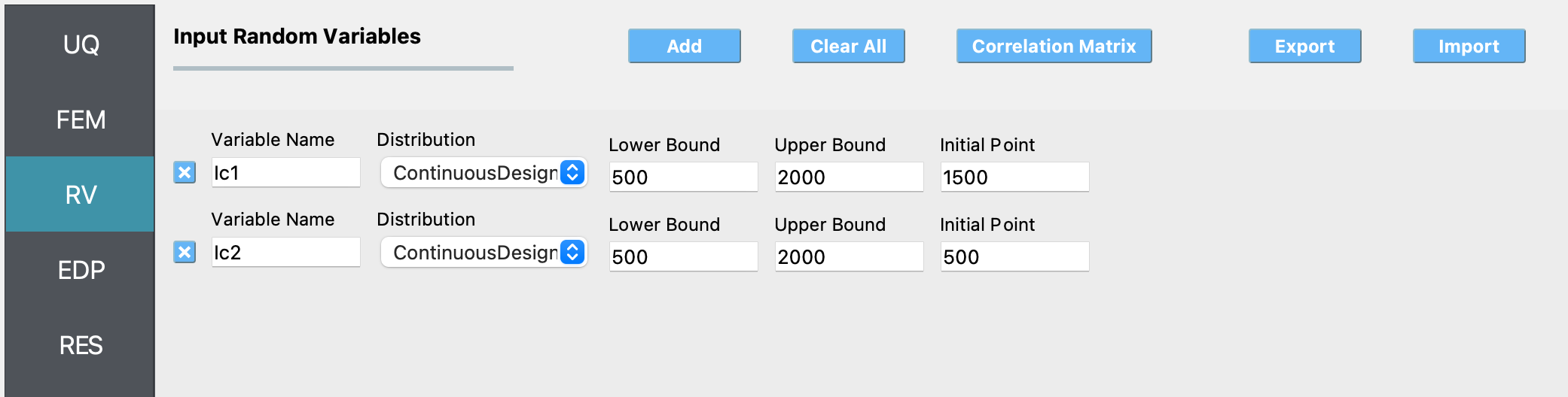
3. Next select the RV tab from the input panel. This should be prepopulated with two random variables with same names as those having pset in the tcl script, i.e. Ic1 and Ic2. For each variable, from the drop down menu change them from having a constant distribution to a continuous design one and then provide the lower bounds, upper bounds and the starting points shown in the figure below.

Note

For the Parameter Estimation category of UQ methods, only continuous design distributions may be entered.

4. Next select the QoI panel. Here enter 2 variable names for the two quantities output from the model.

Note

For this particular problem setup in which the user is not using a postprocessing script, the user may specify any names for the QoI variables. They are only being used by Dakota to return information on the results.

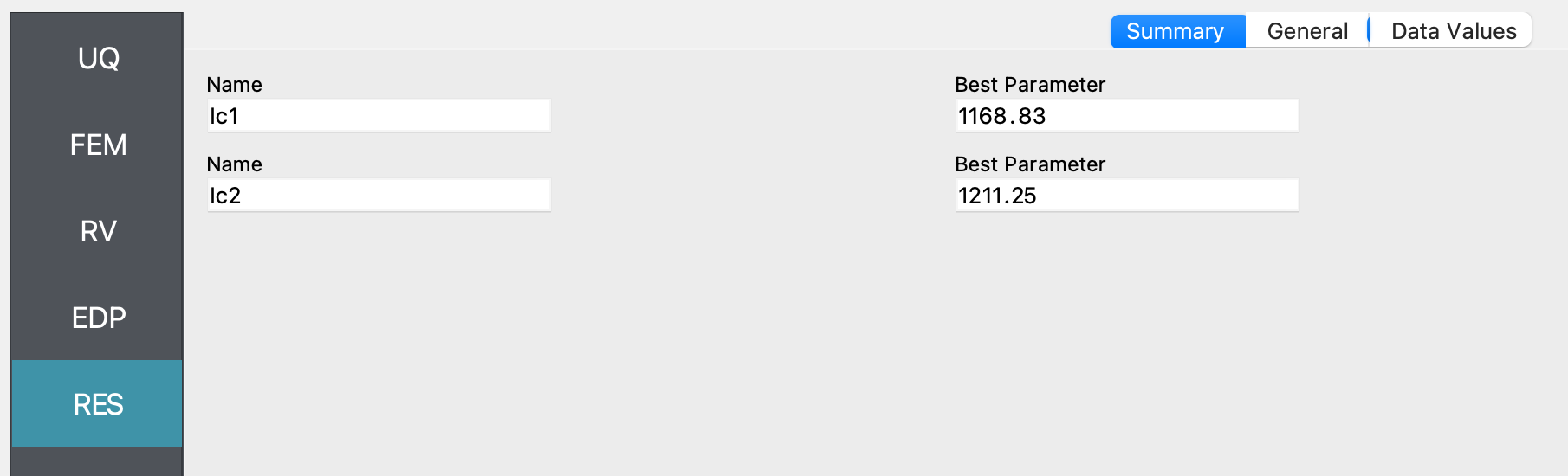
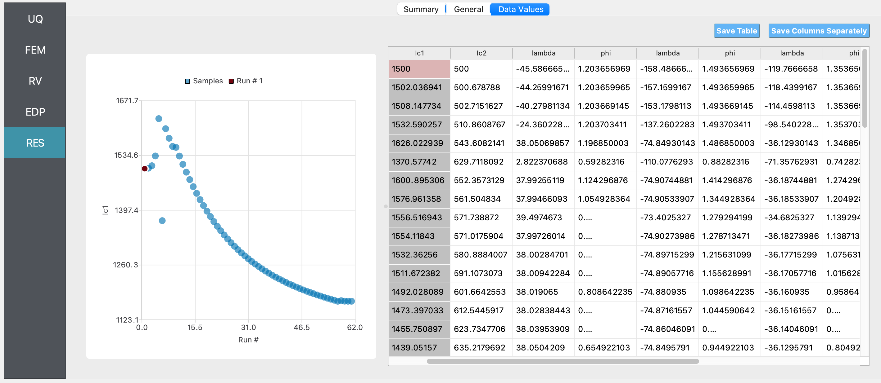
5. Next click on the Run button. This will cause the backend application to launch Dakota. When done the RES tab will be selected and the results will be displayed as shown in the figure below. The figure shows that Dakota estimated the parameters Ic1 and Ic2 as 1168.83 and 1211.25 respectively, for the input data provided. The true value of these parameters, as described in the earlier sections is 1190.