4.8. Surrogate Modeling to Predict Mean and Variance of Earthquake Response

Problem files

Github

4.8.1. Outline

This example constructs a Gaussian process-based surrogate model for mean and standard deviation of a building structure given ten ground motion set.

4.8.2. Problem description

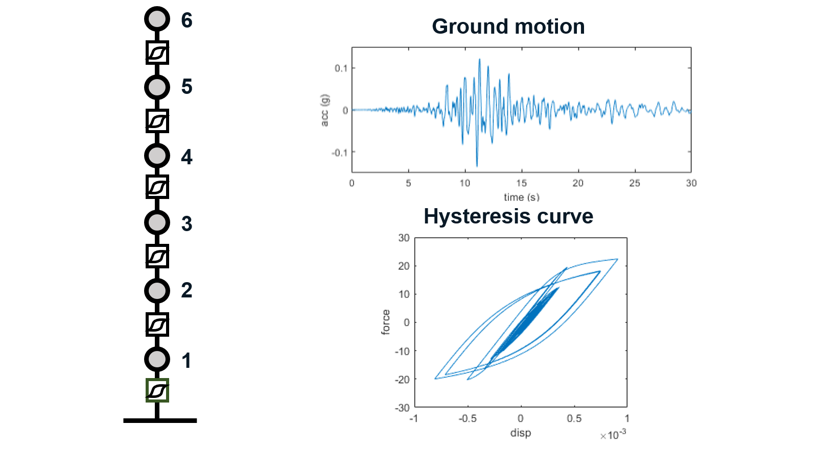
The structure (three story nonlinear building stick model) has the following uncertain properties:

Random Variable	lower bound	upper bound
weight (w)	50	150
roof weight (wR)	40	80
initial stiffness (k)	240	360
post-yield stiff. ratio (alp)	0.05	0.15
yield strength (Fy)	18	22

The goal is to make a surrogate model that predicts mean and standard deviation of the peak displacement at node 1.

4.8.3. Video resources

Note that even though we use the exact same structure, the parameters, their distributions and the quantity of interest (QoI) in the video is different from those in this example. The files for the corresponding example can be found at Github.

Click to replay the video from 26:42. Please note there were minor changes in the user interface since it is recorded.

4.8.4. Input files

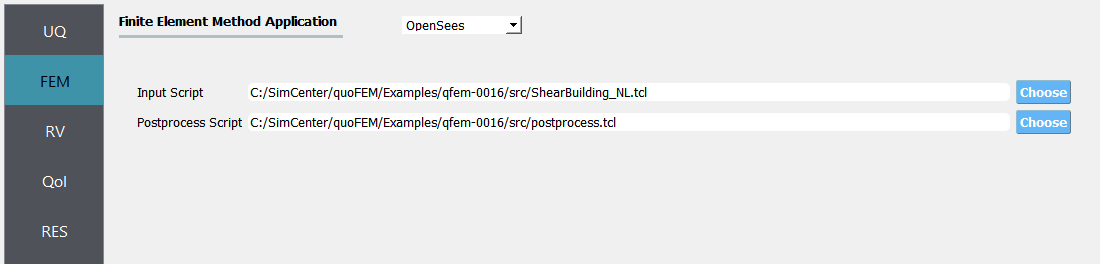
Once the user selects OpenSeesPy as FEM applications, the below two fields are requested.

1. Input Script - ShearBuilding_NL.tcl: This file is the main OpenSees input script that implements builds the model, reads ground motion time histories, and runs the analysis repeatedly. It is supplied to the Input Script field of the FEM tab.

2. Postprocess Script (Optional) - postprocess.tcl: This file is a postprocess script that connects the QoI name to the output value. According to this postprocess file, the QoI should be entered as either in the format of Node_i_Disp_j_Mean or Node_i_Disp_j_Std, where i and j respectively denote the node number and degree of freedom.

The other subsidiary scripts (including ground motion time histories) are stored in the same directory of the main input script.

4.8.5. UQ Workflow

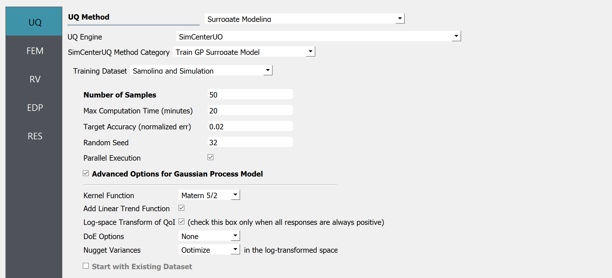
1. Since the model is provided, Training Dataset can be obtained by Sampling and Simulation. Since it is known that the mean and variance of peak drift are always positive, log-transform is introduced. Since a trend is expected, a linear trend function is introduced.

2. Select the FEM tab from the input panel. Choose the engine to be OpenSeesPy. For the main script copy the path name to ShearBuilding_NL.tcl or click choose and navigate to the file. For the postprocess script field, repeat the same procedure for the postprocess.tcl script.

3. Select the RV tab from the input panel. This should be pre-populated with 5 random variables by detecting pset command in ShearBuilding_NL.tcl. For each variable, the distribution option is fixed to be Uniform, and only the lower and upper bounds need to be specified as given in the table.

When the user needs to manually add random variables with add button, eg. when using a custom FEM application, the user should set the distribution to be Uniform using the drop-down menu.

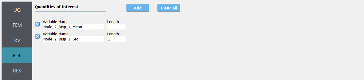
4. Select the QoI tab. Here enter two output names as Node_2_Disp_1_Mean and Node_2_Disp_1_Std. Note that Node_2_Disp_1 means x-direction displacement of second story floor. These QoI names are processed in the postprocess.tcl provided at the FEM tab.

5. Click on the Run button. This will cause the backend application to run SimCenterUQ Engine.

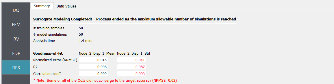
6. When done, the RES tab will be selected and the results will be displayed.

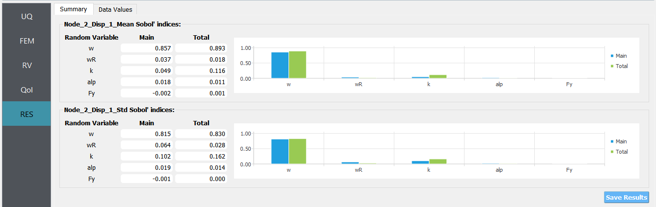
• Summary of Results:

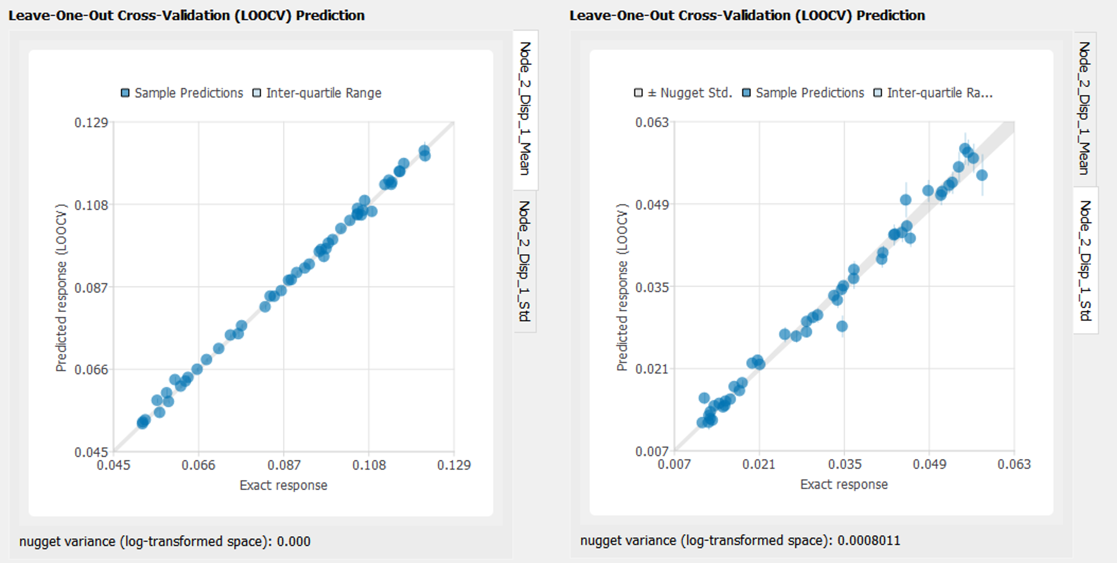
• Leave-one-out cross-validation (LOOCV) predictions:

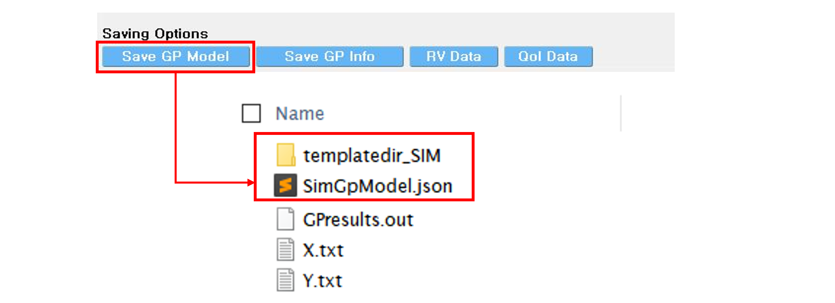
7. Save the surrogate model by clicking Save GP Surrogate

4.8.6. Sensitivity analysis using the Surrogate model

Once the surrogate model is trained, it can be used for various UQ/optimization applications. Here we perform a sensitivity analysis and compare it with the results from simulation model.

1. The constructed surrogate model can be saved by Save GP Model button. Two files and a folder will be saved which are SurroateGP Info File (default name: SimGpModel.json), SurroateGP model file (default name: SimGpModel.pkl) and Simulation template directory which contains the simulation model information (templatedir_SIM).

Note

• Do not change the name of templatedir_SIM. SurrogateGP Info and model file names may be changed.

• When location of the files are changed, templatedir_SIM should be always located in the directory same to the SurroateGP Info file.

Warning

Do not place above surrogate model files in your root, downloads, or desktop folder as when the application runs it will copy the contents on the directories and subdirectories containing these files multiple times. If you are like us, your root, Downloads or Documents folders contains and awful lot of files and when the backend workflow runs you will slowly find you will run out of disk space!

2. Restart the quoFEM (or press UQ tab) and select Dakota sensitivity analysis method.

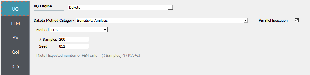
3. Select the FEM tab from the input panel and choose SurrogateGP application. For the SurrogateGP Info field, copy the path to SimGpModel.json or click choose and navigate to the file. Similarly, the SurroateGP Model field calls SimGpModel.pkl file. Once the first file is imported, additional options will be displayed. Here, the user can specify the Maximum Allowable Normalized Variance level. The exceedance percentage is provided to help the user’s decision along with the pre-informed accuracy of the surrogate model obtained after the training session. Select continue to use only surrogate model predictions.

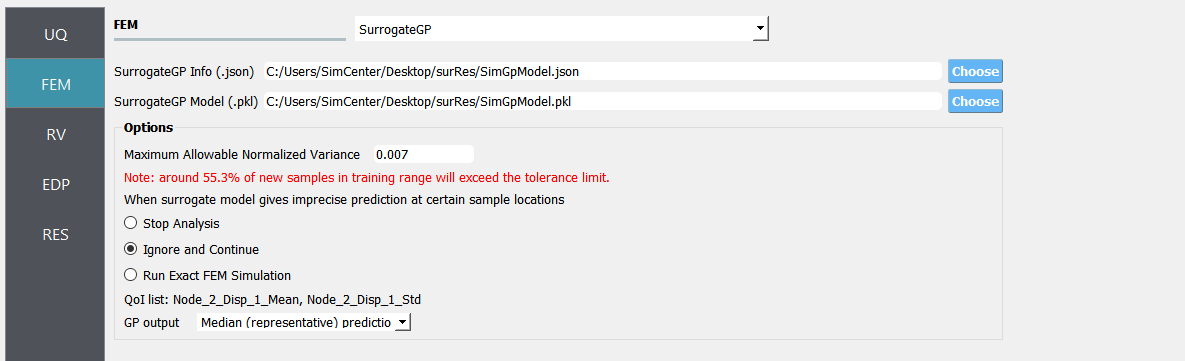
Note

The Continue option should be used only when users are familiar with potential issues.

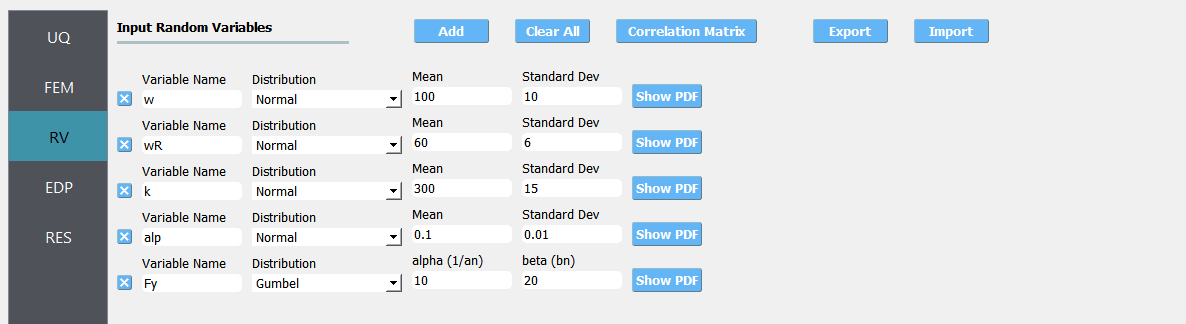
4. Once the SurrogateGP Info field in the FEM tab is entered, the RV tab is automatically populated. The user can select the distribution and its parameters. This example applied the following distributions.

5. Users need to manually fill in the QoI tab. Users do not need to include here all the QoIs used for the training, but the users may not add new QoIs or modify the names of existing QoIs. [Tip] List of the trained QoI names can be found and copied in the FEM tab.

6. Click on the Run button. This will cause the backend application to launch dakota.

7. When done, the RES tab will be selected and the results will be displayed.

• Surrogate model prediction

Surrogate model training time: 1.4 min. (number of FEM runs: 50)

Sensitivity analysis time: 10.3 min. (number of surrogate model evaluations: 1400)

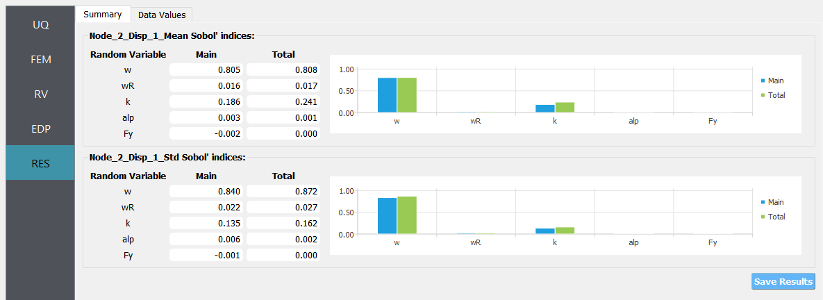
• Reference simulation model results

Sensitivity analysis time: 83.7 min. (number of FEM runs: 1400)