4.11. Two-Dimensional Truss: PLoM Modeling and Simulation

4.11.1. About PLoM

PLoM is an open source python package that implements the algorithm of Probabilistic Learning on Manifolds with and without constraints ([SoizeGhanem2016], [SoizeGhanem2020]) for generating realizations of a random vector in a finite Euclidean space that are statistically consistent with a given dataset of that vector.

PLoM functionality in SimCenter tools is built upon PLoM package (available under MIT license), an opensource python package for Probabilistic Learning on Manifolds [ZhongGualGovindjee2021]. The package mainly consists of python modules and invokes a dynamic library for more efficiently computing the gradient of the potential, and can be imported and run on Linux, macOS, and Windows platform.

4.11.2. Problem Statement

Consider the problem simulating response of a two-dimensional truss structure with uncertain material properties shown in the following figure. The goal of the exercise is to demonstrate the use of PLoM model method under SimCenterUQ.

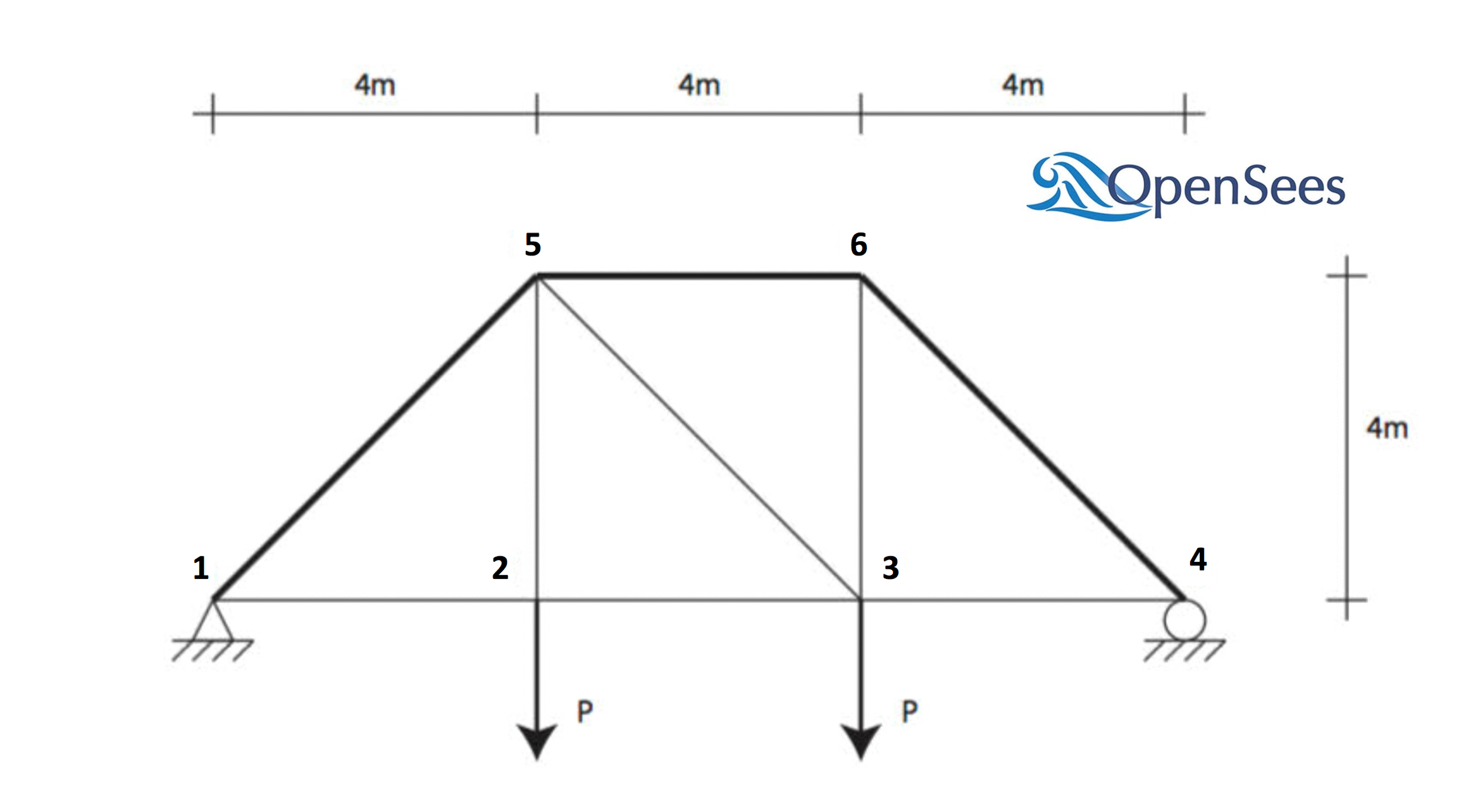
1. Elastic modulus(E): mean \(\mu_E=205 kN/{mm^2}\) and standard deviation \(\sigma_E =15 kN/{mm^2}\) (COV = 7.3%)

2. Load (P): mean \(\mu_P =25 kN\) and a standard deviation of \(\sigma_P = 3 kN\), (COV = 12%).

3. Cross sectional area for the upper three bars (Au): mean \(\mu_{Au} = 500 mm^2\), and a standard deviation of \(\sigma_{Au} = 25mm^2\) (COV = 5%)

4. Cross sectional area for the other six bars (Ao): mean \(\mu_{Ao} = 250mm^2\), and \(\sigma_{Ao} = 10mm^2\) (COV = 4%)

The exercise requires two files:

1. TrussTemplate.tcl

# units kN & mm

#
# set some parameters
#

pset E 205
pset P 25
pset Au 500
pset Ao 250

#
# build the model
#

model Basic -ndm 2 -ndf 2

node 1     0    0
node 2  4000    0
node 3  8000    0
node 4 12000    0
node 5  4000 4000
node 6  8000 4000

fix 1 1 1
fix 4 0 1

uniaxialMaterial Elastic 1 $E

element truss 1 1 2 $Ao 1
element truss 2 2 3 $Ao 1
element truss 3 3 4 $Ao 1
element truss 4 1 5 $Au 1
element truss 5 5 6 $Au 1
element truss 6 6 4 $Au 1
element truss 7 2 5 $Ao 1
element truss 8 3 6 $Ao 1
element truss 9 5 3 $Ao 1
timeSeries Linear 1
pattern Plain 1 1 {
    load 2 0 [expr -$P]
    load 3 0 [expr -$P]
}

#
# create a recorder
#

recorder Node -file node.out -scientific -precision 10 -node 1 2 3 4 5 6 -dof 1 2 disp

#
# build and perform the analysis
#

algorithm Linear
integrator LoadControl 1.0
system ProfileSPD
numberer RCM
constraints Plain
analysis Static
analyze 1

#
# remove the recorders
#

remove recorders

2. TrussPost.tcl.

The TrussPost.tcl script shown below will accept as input any of the 6 nodes in the domain and for each of the two dof directions.

# create file handler to write results to output & list into which we will put results
set resultFile [open results.out w]
set results []

# get list of valid nodeTags
set nodeTags [getNodeTags]

# for each quanity in list of QoI passed
#  - get nodeTag
#  - get nodal displacement if valid node, output 0.0 if not
#  - for valid node output displacement, note if dof not provided output 1'st dof

foreach edp $listQoI {
	set splitEDP [split $edp "_"]	
	set nodeTag [lindex $splitEDP 1]
	if {$nodeTag in $nodeTags} {
	    set nodeDisp [nodeDisp $nodeTag]
	    if {[llength $splitEDP] == 3} {
		set result [expr abs([lindex $nodeDisp 0])]
	    } else {
		set result [expr abs([lindex $nodeDisp [expr [lindex $splitEDP 3]-1]])]
	    }
	} else {
	    set result 0.
	}
	lappend results $result
}

# send results to output file & close the file
puts $resultFile $results
close $resultFile

4.11.3. PLoM Modeling

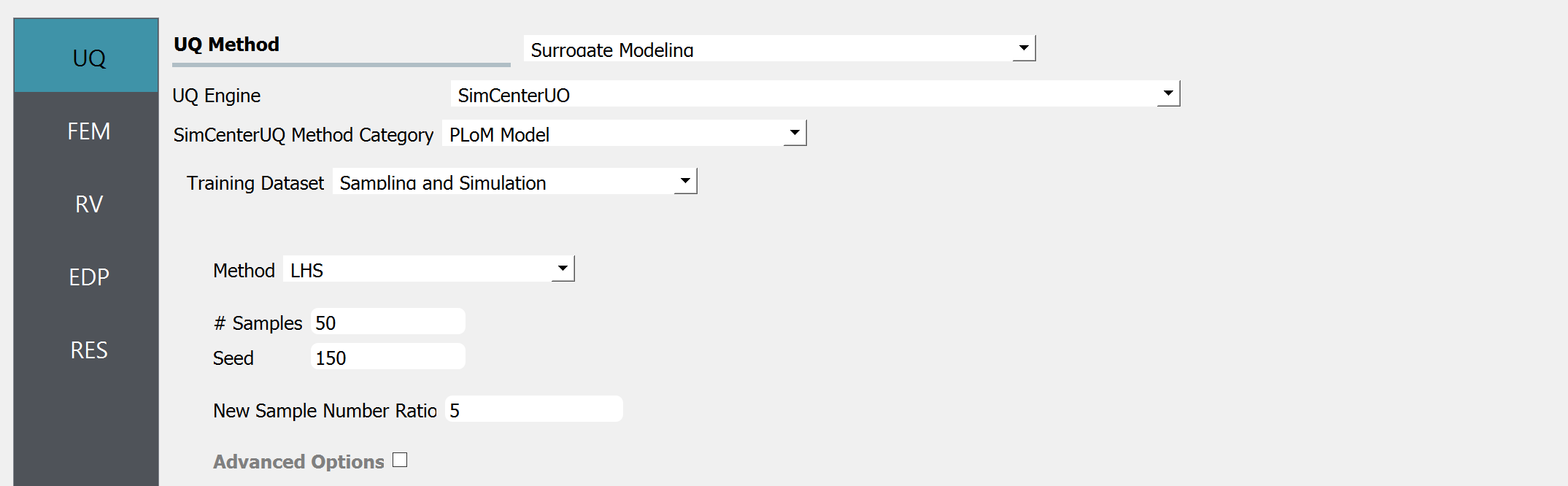
1. Start the application and the UQ Selection will be highlighted. In the panel for the UQ selection, select SimCenterUQ as the UQ engine. Select PLoM Model for the UQ method, and use Sampling and Simulation as the Training Dataset. For sampling method, select LHS with 50 initial simulations for generating training data (with a random seed specified). For the new sample number ratio, input 5 by which 250 new realizations will be created from the trained PLoM model.

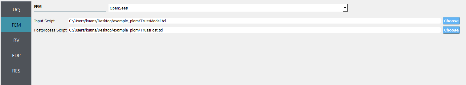
2. Next select the FEM panel from the input panel. This will default in the OpenSees engine. For the main script copy the path name to TrussModel.tcl or select choose and navigate to the file. For the post-process script field, repeat the same procedure for the TrussPost.tcl script.

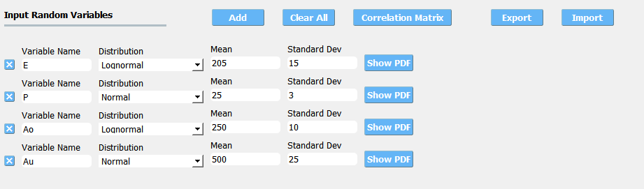
3. Next select the RV panel from the input panel. This should be pre-populated with four random variables with same names as those having pset in the tcl script. For each variable, from the drop down menu change them from having a constant distribution to a normal one and then provide the means and standard deviations specified for the problem.

4. Next select the EDP tab. Here two response variables Node_2_Disp_2 and Node_3_Disp_2 are defined, which should be consistent with the post-process script.

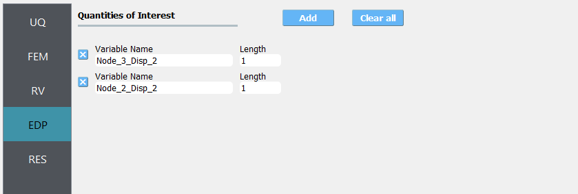
Note

The user can add extra EDP by selecting add and then providing additional names. As seen from the post-process script any of the 6 nodes may be specified and for any node either the 1 or 2 DOF direction.

5. Next click on the Run button. This will cause the backend application to launch the job. When done the RES panel will be selected and the results will be displayed. The landing page of RES will show summarize the training information including training sampling number along with two PLoM model trucation plots for PCA and KDE.

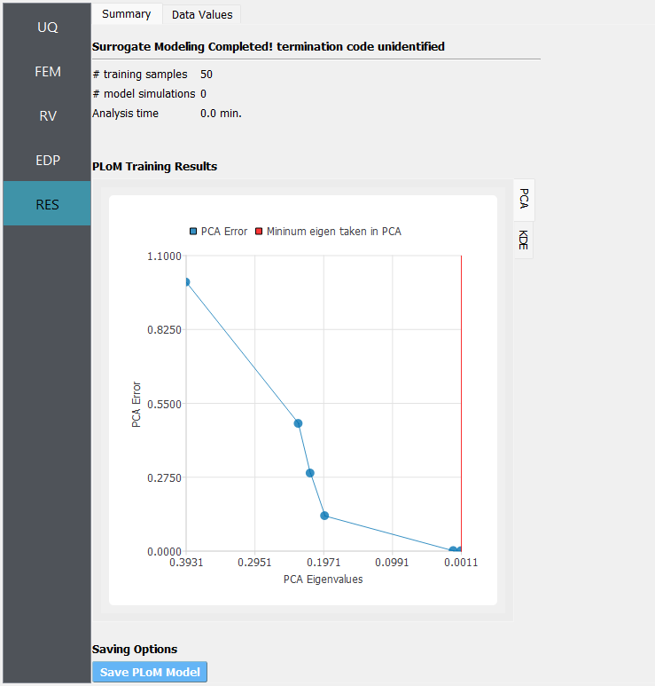
Fig. 4.11.3.1 PCA representation error versus the PCA eigenvalues overlapped by the truncating PCA eigenvalue used in training

Fig. 4.11.3.2 Diffusion map eigenvalue by components overlapped by the truncating eigenvalue used in training

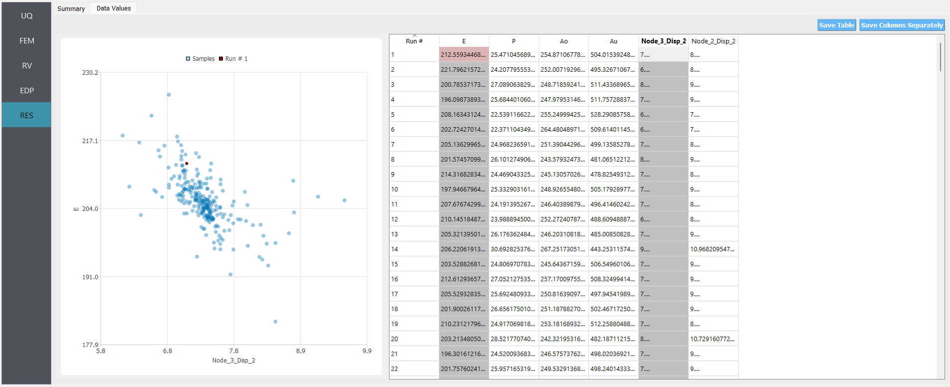
If the user selects the Data tab in the results panel, they will be presented with both a graphical plot and a tabular listing of the data. Various views of the graphical display can be obtained by left and right clicking in the columns of the tabular data. If a singular column of the tabular data is pressed with both right and left buttons a frequency and CDF will be displayed, as shown in figure below.

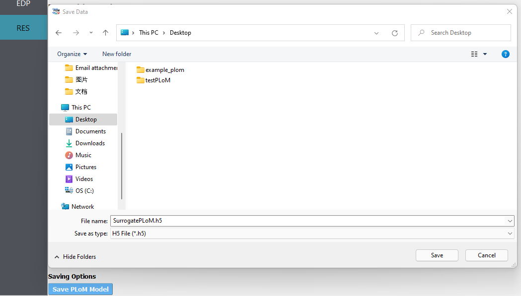
The PLoM model can be saved and be loaded back for future use. The Save PLoM Model button at the bottom of Summary page would bring up a dialogue window for saving the model file to a user-defined directory.

SoizeGhanem2016

Soize, C., & Ghanem, R. (2016). Data-driven probability concentration and sampling on manifold. Journal of Computational Physics, 321, 242-258.

SoizeGhanem2020

Soize, C., & Ghanem, R. (2020). Physics-constrained non-Gaussian probabilistic learning on manifolds. International Journal for Numerical Methods in Engineering, 121(1), 110-145.

ZhongGualGovindjee2021

Zhong, K., Gual, J., and Govindjee, S., PLoM python package v1.0, https://github.com/sanjayg0/PLoM (2021).