4.13. Heteroscedastic Gaussian Process modeling

Problem files

Github

4.13.1. Outline

In this example, demonstrates the heteroscedastic Gaussian process model for surrogating noisy response.

4.13.2. Problem description

Let us consider the basic python model in this example with fixed \(y=0\).

(4.13.2.1)\[g(x)=(a-x)^{2}+bx^{4}+\varepsilon\]

where \(\varepsilon\) is an additive Gaussian noise that represent the variability in the output response surface. Let us assume \(\varepsilon\) has zero mean and non-homogeneous variance of \(\sigma(x)^2 = (x+2.0)^2\).

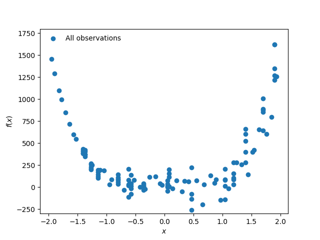
Fig. 4.13.2.1 Observation dataset

We would like to create a surrogate model of this function for the input range of \(x\in[-2,2]\)

4.13.3. Files required

The exercise requires one main script file and one supplementary file. The user should download these files and place them in a NEW folder.

Warning

Do NOT place the files in your root, downloads, or desktop folder as when the application runs it will copy the contents on the directories and subdirectories containing these files multiple times. If you are like us, your root, Downloads or Documents folders contains a lot of files.

1. rosenbrock.py - This is a python script that computes the model. The script is based on this example, but with \(y=0\). Further, \(\varepsilon(x)\) is generated using numpy random sampler.

   Listing 4.13.3.1 rosenbrock.py

   #!/usr/bin/python
   
   # written: adamzs 06/20
   # The global minimum is at (a, a^2)
   
   import sys
   import numpy as np
   from params import *
   import os
   def rosenbrock(x, y):
   	
   	np.random.seed(int(os.getcwd().split("workdir.",1)[1])) # to make this example reroducable. 
   	# different working directories should take DIFFERENT random seed.
   
   	a = 1.
   	b = 100.
   	eps = 50*np.random.normal(loc=0.0, scale=1.0, size=None)
   	print(eps)
   	return (a - x)**2. + b*(y - x**2.)**2 + eps*(x+2.0)
   
   if __name__ == "__main__":
   
   	Y = 0.0 # deterministic variable
   	with open('results.out', 'w') as f:
   		result = rosenbrock(X, Y)
   		f.write('{:.60g}'.format(result))
   
   

2. params.py- This file defines the input variable(s) that the surrogate model will take

   Listing 4.13.3.2 params.py

   X = 0.0
   

Note

Since the python script creates a results.out file when it runs, no postprocessing script is needed.

4.13.4. UQ workflow

The steps involved are as follows:

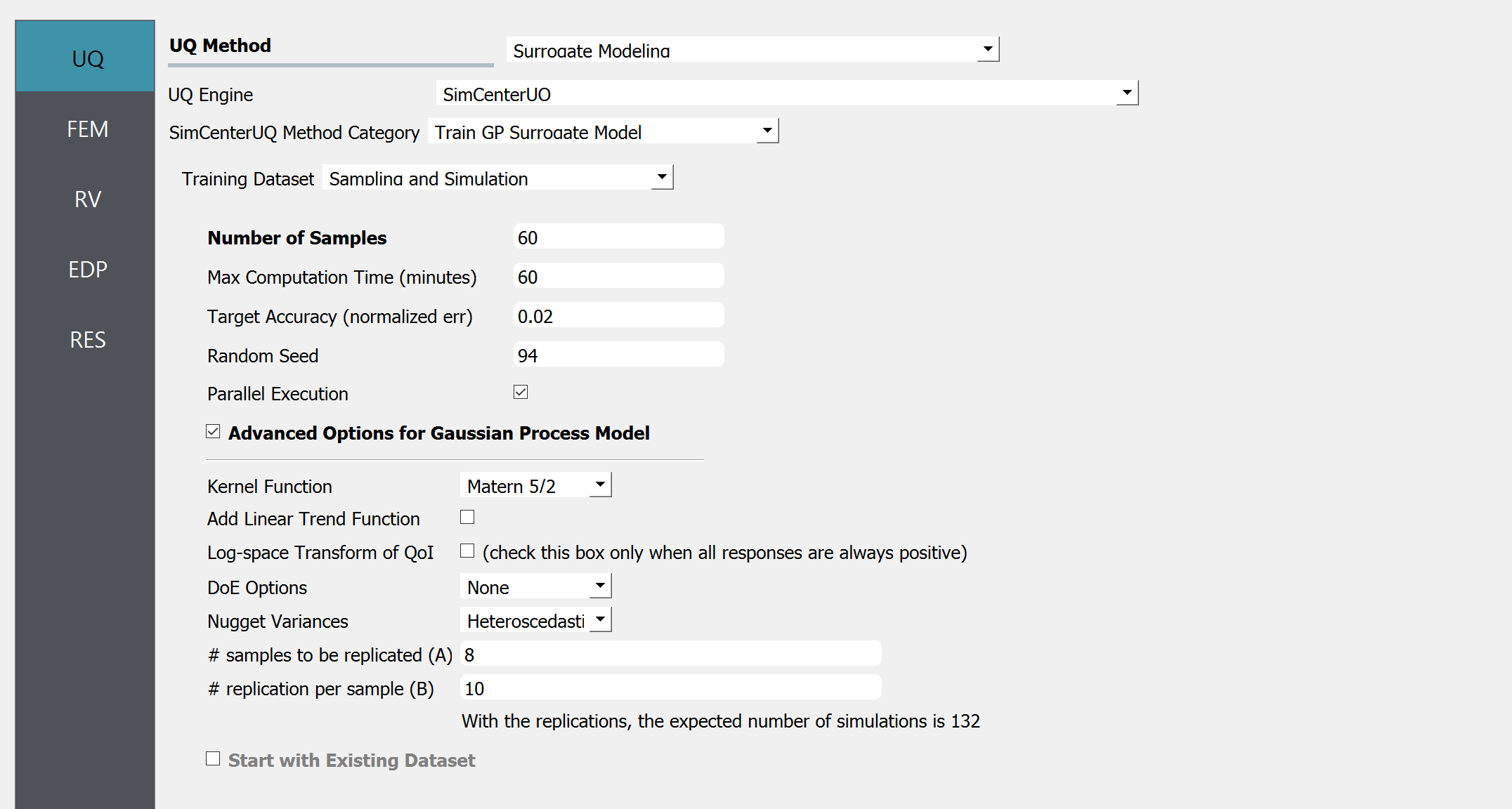
1. Start the application and the UQ panel will be highlighted. In the UQ Engine drop down menu, select the SimCenterUQ engine. In the Method select Train GP Surrogate option. Enter the values in this panel as shown in the figure below.

2. Next in the FEM panel , select Python FEM engine. Enter the paths to the rosenbrock.py and params.py or select Choose and navigate to the files.

Note

Since the python script creates a results.out file when it runs, no postprocessing script is needed.

3. Select the RV tab from the input panel. This panel should be pre-populated with \(x\). If not, press the Add button to create a new field to define the input random variable. Enter the same variable name, as required in the model script. Specify the input range of interest

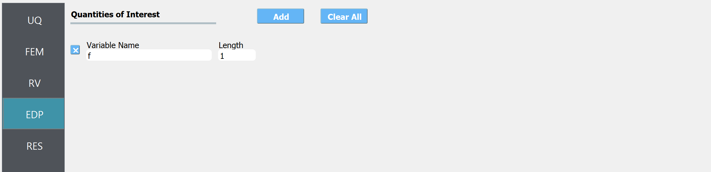
4. In the QoI panel enter a variable named f with length 1.

5. Click on the Run button. This will cause the backed application to launch the SimCenterUQ engine, which performs the surrogate training.

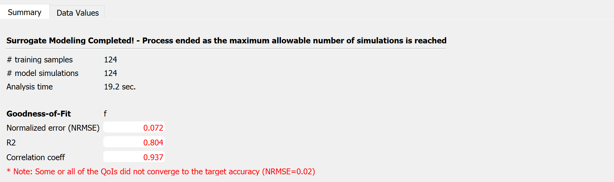
6. When done, the RES tab will be selected and the results will be displayed.

• Summary of Results:

• Leave-one-out cross-validation (LOOCV) predictions:

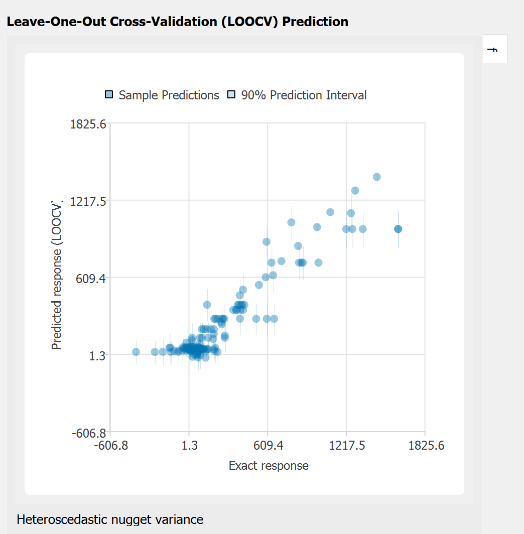
Note that the goodness-of-fit measures above do not perfectly capture goodness as it is evaluated assuming aleatory variability (or the measurement noise) zero. However, the cross-validation plot with bounds provides a rough estimate of whether the observation data safely lies on the GP prediction bounds. A better validation measure for the case with high nugget variance will be included in the next release.

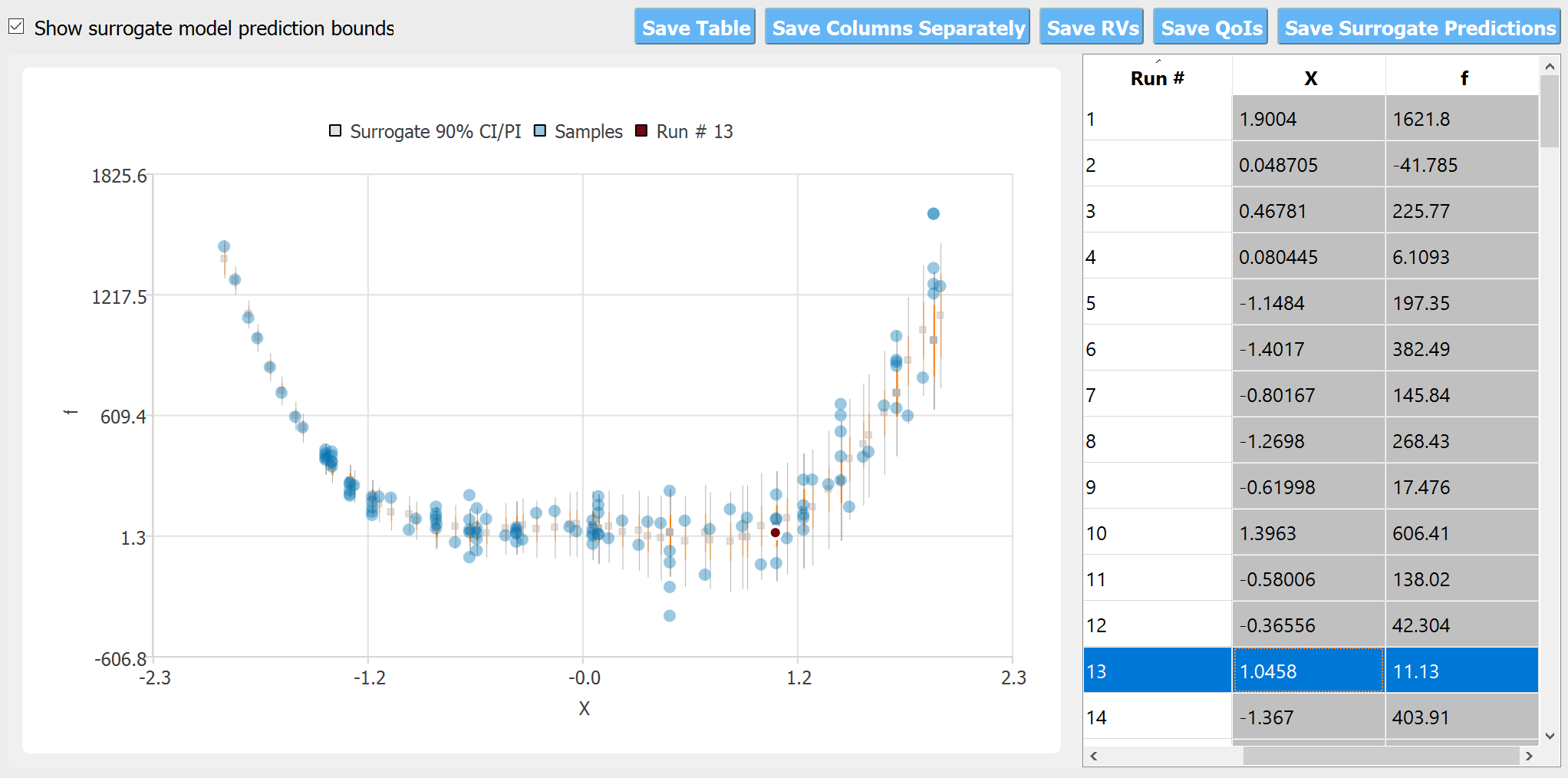
The scatter plot compares the observation data with the predicted mean and variance obtained by cross-validations. The confidence interval (CI, shown in red) is the bounds for the ‘mean’ of the response function, while the prediction interval (PI, shown in gray) shows those of the observations (i.e. by adding the range of the measurement noise)