5.3. Regional Site Response Assessment

5.3.1. Problem Statement

Site response analysis is commonly performed to analyze the propagation of seismic wave through soil. As shown in Fig. 2.3.5.1, one-dimensional response analyses, as a simplified method, assume that all boundaries are horizontal and that the response of a soil deposit is predominately caused by SH-waves propagating vertically from the underlying bedrock. Ground surface response is usually the major output from these analyses, together with profile plots such as peak horizontal acceleration along the soil profile. When liquefiable soils are presenting, maximum shear strain and excess pore pressure ratio plots are also important.

Fig. 5.3.1.1 Simplified 1D site response analysis (courtesy of Pedro Arduino)

This example demonstrates a small-scale regional earthquake risk assessment which performs site response simulation for a group of 20 sites located in the San Francisco Bay area. The sites are distributed in space in a 4x5 grid, within a 3x3 grid of event sites. At each event site, 5 ground motion records of similar intensity are assigned.

Fig. 5.3.1.2 Location of testbed sites

5.3.2. Methodology

In this example, the coordinates of a list of sites are known and peak ground accelerations at these sites are of interest. A summary of the RDT procedure for the site response analysis is summarized here:

1. Assemble required information for interested sites. These data include site locations, input motions, and site geological data, e.g., Vs30 (the time-averaged shear-wave velocity to 30 m depth) and depth to bedrock

2. If the input motions are not provided, use OpenSHA to obtain proper input motions

3. If the Vs30 data are not known, use SimCenter EQHazard to obtain proper Vs30 data

4. If the depth to bedrock data are not known, they can be obtained from SoilGrid250 database

5. Use Sediment Velocity Model (SVM) to generate soil shear wave velocity profile

6. Generate material input for site response analysis based on predefined model calibration methods

7. Perform site response analysis using RDT and obtain acceleration response at the surface of soil columns defined for each site

In this example, a total of twenty sites and their input motions have been pre-selected. Details of selected sits are summarized in tab_inputs. The directory structure for inputs is:

srt_example
├── rWHALE_config_SRT.json
└── input_data
    ├── model
        ├── getVs30.py
        ├── Scenario.json
        ├── FreeField3D_Dry.tcl
    ├── records
        ├── EventGrid.csv
        ├── RSN30.json
        ├── RSN63.json
        .
        .
        .
        ├── site0.csv
        ├── site1.csv
        .
        .
        .
        └── site8.csv
    └── input_params.csv

5.3.2.1. Obtaining Vs30 Data

Vs30 data can be obtained using EQHazard tool. EQHazard is a console application developed by the SimCenter to facilitate performing seismic hazard analysis(SHA) for regional earthquake simulations. The application makes use of OpenSHA to perform deterministic SHA. This application is developed using Java to facilitate the use of OpenSHA Java library. It is worth noting that this tool is most suitable for research applications where SHA needs to be performed for many sites given a single earthquake scenario, such as using a grid of sites for regional simulations. Several site data sources have been included in EQHazard, such as CGS/Wills VS30 Map (2015), Global Vs30 from Topographic Slope (Wald & Allen 2008), and more.

Using EQHazard is simple, the EQHazard tool is distributed as a jar file and can executed directly using:

java -jar EQHazard Scenario.json Output.json

Scenario.json is the name of the input file and output.json is the name to be used for the resulting output file.

Note

Java is required to run EQHazard

Python script getVs30.py provides a wrapper for EQHazard. It uses the site coordinates from input_params.csv and a template scenario file, Scenario.json, to obtain Vs30 data. An updated input file, input_params_srt.csv, is then created with Vs30 data populated as shown in Table 5.3.2.1.1. In this case, CGS/Wills VS30 Map (2015) is used.

Table 5.3.2.1.1 Input Parameters with Vs30 Data Obtained Using EQHazard

id	longitude	latitude	stories	yearbuilt	occupancy	structure	areafootprint	replacementCost	W	f_yield	T1	Vs30	DepthToRock
0	-122.182	37.422	0	1957	RES1	W1	1293.253476	1	55.25	118.75	0.29375	386.6	7.61
1	-122.18575	37.422	0	1927	RES1	W1	2568.835761	1	86.75	148.75	0.15625	386.6	8.79
2	-122.1895	37.422	0	2020	RES1	W1	1127.07738	1	114.75	123.75	0.39375	351.9	9.28
3	-122.19325	37.422	0	1951	RES1	W1	2085.809768	1	107.75	126.25	0.24375	386.6	8.65
4	-122.197	37.422	0	1960	RES1	W1	1481.567067	1	76.25	101.25	0.30625	386.6	7.74
5	-122.182	37.42366667	0	1986	RES1	W1	1240.719532	1	90.25	116.25	0.21875	386.6	7.65
6	-122.18575	37.42366667	0	1984	RES1	W1	2437.970509	1	93.75	141.25	0.35625	386.6	9.35
7	-122.1895	37.42366667	0	1983	RES1	W1	2668.60615	1	111.25	133.75	0.36875	351.9	9.88
8	-122.19325	37.42366667	0	1957	RES1	W1	1553.47035	1	104.25	108.75	0.19375	386.6	9.71
9	-122.197	37.42366667	0	1984	RES1	W1	1625.164708	1	58.75	106.25	0.23125	386.6	9.32
10	-122.182	37.42533333	0	2018	RES1	W1	1787.865419	1	62.25	143.75	0.34375	386.6	7.53
11	-122.18575	37.42533333	0	2018	RES1	W1	1821.174819	1	65.75	138.75	0.20625	386.6	9.02
12	-122.1895	37.42533333	0	1930	RES1	W1	1624.532488	1	69.25	146.25	0.31875	386.6	9.79
13	-122.19325	37.42533333	0	1922	RES1	W1	1134.673241	1	79.75	103.75	0.25625	351.9	9.84
14	-122.197	37.42533333	0	1947	RES1	W1	1625.097354	1	51.75	128.75	0.16875	386.6	10.67
15	-122.182	37.427	0	1969	RES1	W1	2289.96328	1	83.25	131.25	0.33125	386.6	7.66
16	-122.18575	37.427	0	2006	RES1	W1	2288.360712	1	100.75	136.25	0.38125	386.6	9.77
17	-122.1895	37.427	0	1959	RES1	W1	2291.605647	1	97.25	111.25	0.18125	351.9	9.8
18	-122.19325	37.427	0	1979	RES1	W1	2770.811412	1	72.75	113.75	0.26875	351.9	10.03
19	-122.197	37.427	0	1976	RES1	W1	2088.450773	1	118.25	121.25	0.28125	386.6	9.68

5.3.2.2. Obtaining Depth to Bedrock

The depth to bedrock can be obtained using several datasets. For example, SoilGrid250 map provides absolute depth to bedrock (in cm) predicted using the global compilation of soil ground observations. Accuracy assessment of the maps is available in Hengl [] and can be downloaded here. In this dataset, the depth to bedrock is considered as “depth (in cm) from the ground surface to the contact with coherent (continuous) bedrock.” It should be noted that the definition of bedrock in this database is based on lithology rather than shear wave velocity. Hence, depending on the geological condition, bedrock may imply different shear wave velocity and it might vary dramatically, e.g., western U.S. vs. eastern U.S.. Assumption is required for modeling purposes. In this example, the shear wave velocity of bedrock is assumed to be 760 m/s, as the sites are located in western U.S..

Fig. 5.3.2.2.1 Depth to bedrock (Cropped from SoilGrid250 to show continental U.S., 10 km resolution)

Example python script to obtain the data is shown below:

import rioxarray as rxr
import pandas as pd
from pyproj import Transformer

soil250 = rxr.open_rasterio('BDTICM_M_250m_ll.tif')
inputs = pd.read_csv('input_params_srt.csv')
for index, row in inputs.iterrows():
   lon = row['longitude']
   lat = row['latitude']
   transformer = Transformer.from_crs("EPSG:4326", soil250.rio.crs, always_xy=True)
   xx, yy = transformer.transform(lon, lat)
   depth_To_Rock = soil250.sel(x=xx, y=yy, method="nearest").values[0]
   print('depth to rock is {:.2f} m'.format(depth_To_Rock/100))

5.3.2.3. Generating Soil Profile Using SVM

Once the depth to rock is obtained, the next step is to generate soil profile based on Vs30. Amplitude, frequency content and duration of ground shaking are important parameters in ground motion modeling and are heavily dependent on crustal material properties. The Sediment Velocity Model (SVM) “translates VS30 and a proxy which describes stiffness of the near surface sediments into a 1D velocity profile” (Shi and Asimaki, 2018, []).

Datasets of soil parameters only exist for specific locations and there is no way to collect adequate data on all regions. For this reason, there is a need for a method which can determine these crustal material properties such as wave velocity and mass density for those regions which we do not have physically collected data. One such method, called the Community Velocity Models (CVMs), which was developed by the Southern California Earthquake Center (SCEC), is used to provide 3D seismic velocity information for Southern California. However, CVMs have their limitations. There exist two sub-models of the CVM which are the CVM-SCEC (CVM-S) and CVM-Harvard (CVM-H). Both sub-models rely on the spatial resolution of the available datasets and thus result in crude velocity profiles. Moreover, the CVM-H has an optional geotechnical layer (GTL) option which replaces the soft sediments in the top 350 m of soil, smoothing the velocity profile and obscuring basin edges which cause strong velocity impedance.

The SVM method was developed to get more accurate soil profiles as a function of VS30 which can be easily obtained from maps. It further allows for determination of basin depths based on crustal velocity models and preserves basin edges.

The Shi and Asimaki [] Sediment Velocity Model (SVM) is used in this example because of its ability to predict a soil velocity profile based solely on VS30. From this profile we are able to determine ground motion wavelengths and set a constraint for a minimum number of points needed to fully describe a soil column. Gmax at depth is also obtained from this shear wave velocity profile. The results of the test case are presented in Fig. 5.3.2.3.1.

Fig. 5.3.2.3.1 Generated shear wave velocity profile based on SVM

5.3.2.4. Including Soil Nonlinearity

By default, elastic isotropic material is assigned to the soil column due to limited available information. However, Nonlinearity can be incorporated into workflow by switching the constitutive model to other nonlinear model, for example, the multiaxial cyclic plasticity model proposed by Borja and Amies []. This simple total stress-based bounding surface plasticity model for clays was developed to accommodate multiaxial stress reversals. The model was constructed based on the idea of a vanishing elastic region undergoing pure translation inside a bounding surface, and an interpolation function for hardening modulus which varies with stress distance of the elastic region from the unloading point. The model can be applied to cohesive soils undergoing undrained stress reversals and cyclic loading. Fig. 5.3.2.4.1 illustrates behaviors of this model under cyclic loading. More information regarding the implementation of this model in OpenSees can be found here.

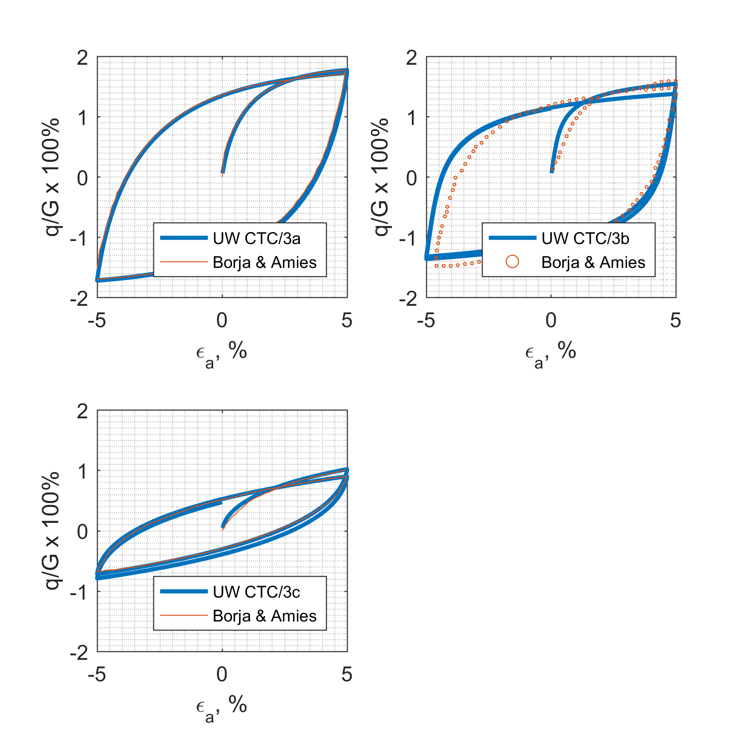
Fig. 5.3.2.4.1 Example behavior of Borja and Amies model

Table 5.3.2.4.1 Input for elastic material

id	longitude	latitude	…	Model
0	-122.182	37.422	…	Elastic

The example input parameters for using Borja and Amies are summarized in the following table:

Table 5.3.2.4.2 Input for multiaxial cyclic plasticity model for clays (Borja and Amies, [])

id	longitude	latitude	…	Model	Su_rat	Den	h/G	m	h0	chi
0	-122.182	37.422	…	BA	0.26	2	1	1	0.2	0

where Su_rat is the ratio between undrain shear strength and initial vertical stress.

5.3.2.5. Adding Surface Structural Model

A structure model can also be added to the workflow. In this case, the structure model uses the OpenSeesPyInput modeling application as discussed in Earthquake Assessment. The buildings are modeled as elastic-perfectly plastic single-degree-of-freedom (SDOF) systems defined by three input model parameters: the weight W, yield strength f_yield, and fundamental period T1. Functions are included which record the peak response as EDPs for each of the EDP types specified in the EDP_specs.json file.

"Modeling": {
"Application": "OpenSeesInputSRT",
"ApplicationData": {
   "mainScript": "FreeField3D_Dry.tcl",
   "modelPath": "model/",
   "ndm": 3,
   "includeStructureModel": true,
   "SimulationApplication": "OpenSeesPy-Simulation",
   "structureModel": "cantilever.py"
}

5.3.2.6. Performing Analysis

Configurations for RDT workflow are defined in rWHALE_config_SRT.json. In this example, the application for Modeling and Simulation is OpenSeesInputSRT and OpenSees-Simulation-SRT, respectively.

For each site, two additional input files for OpenSees are created during analysis: freefield_config.tcl and freefield_material.tcl. freefield_config.tcl defines the discretization of the profile and applied input motion(s).

# site response configuration file
set soilThick 99.0
set numLayers 198
# layer thickness - bottom to top
set layerThick(1) 0.50
set nElemY(1) 1
set sElemY(1) 0.500
set layerThick(2) 0.50
set nElemY(2) 1
set sElemY(2) 0.500

# ...
# ...

# motion file (used if the input arguments do not include motion)
set accFile  xInput.acc
set dispFile xInput.disp
set velFile  xInput.vel
set timeFile xInput.time
set numEvt 2
set accFile2  yInput.acc
set dispFile2 yInput.disp
set velFile2  yInput.vel
set rockVs 760.0
set omega1 8.59
set omega2 42.95

freefield_material.tcl defines material inputs based on predefined calibration procedure based on Vs profile created from previous step. Input motion(s) is converted from records for each evaluation, for example, xInput.vel and xInput.time defiles velocity and time series, respectively, for one component of the motion.

set rho(1) 2.0
set shearG(1) 112692.20
set nu(1) 0.30
set E(1) 292999.71

set mat(1) "ElasticIsotropic 1 $E(1) $nu(1) $rho(1)"


set rho(2) 2.0
set shearG(2) 112692.20
set nu(2) 0.30
set E(2) 292999.71

set mat(2) "ElasticIsotropic 2 $E(2) $nu(2) $rho(2)"

# ... 
# ...

The working/results directory structure is:

results
   └── 0
      ├── templatedir
         ├── bim.j
         ├── edb.j
         |── evt.j
         ├── sam.j
         ├── workflow_driver.bat
      ├── workdir.1
         ├── FreeField3D_Dry.tcl
         ├── freefield_config.tcl
         ├── freefield_material.tcl
         ├── xInput.vel
         ├── xInput.time
         ├── yInput.vel
         ├── yInput.time
         .
         .
         .
      ├── workdir.2
      .
      .
      ├── workdir.5
      └── response.csv
   └── 1
   .
   .
   └── 19

EDP_1-19.csv: reports statistics on the EDP results from simulating 5 ground motions for each building asset. The statistics reported are the median and lognormal standard deviation of peak ground acceleration (shown as PFA) in two directions.

Table 5.3.2.6.1 EDP Results

type	PGA	PGA	PGA	PGA
loc	0	0	0	0
dir	1	1	2	2
stat	median	beta	median	beta
0	0.6628029999999999	0.13600449843043236	0.736927	0.1275636943053479
1	0.633193	0.20304404095647471	0.717512	0.24904764429936244
2	0.721433	0.38880051595831655	0.715938	0.3514059337674102
3	0.713946	0.14054739273872968	0.764877	0.3915961386798949
4	0.743542	0.2171580362193277	0.49029799999999996	0.2407229856374786
5	0.6505810000000001	0.15337053057961506	0.56929	0.19106712482954594
6	0.667912	0.0821461264634056	0.76647	0.2854761912873225
7	0.8115100000000001	0.3580416351456673	0.7321770000000001	0.10374091963523832
8	0.5919449999999999	0.484515336289696	0.767825	0.2795311183002603
9	0.8206610000000001	0.169420903616953	0.679726	0.31719489352530283
10	0.6627770000000001	0.1160975874275244	0.623636	0.1383857442038908
11	0.664215	0.3068794966334912	0.681191	0.17780768288420262
12	0.7623260000000001	0.3342121915707141	0.709516	0.10729744618054217
13	0.540041	0.2794970883918737	0.702222	0.07850396436049084
14	0.628897	0.3682471518218779	0.6626449999999999	0.08292658813669537
15	0.63932	0.3279279372030125	0.574796	0.2115260225991987
16	0.74392	0.3603316789411304	0.690448	0.21550453311227016
17	0.8111510000000001	0.2871611406223856	0.714084	0.20898183490987293
18	0.6592899999999999	0.3766289667049084	0.742772	0.11470562563412998
19	0.67061	0.17423255167006754	0.740329	0.3700796708017528

Under Windows system, the commands can be summarized as:

5.3.3. Appendix

Configurations for RDT workflow:

{
  "Name": "rWHALE_",
  "Author": "Adam Zsarnóczay",
  "WorkflowType": "Parametric Study",
  "buildingFile":"buildings.json",
  "runDir": "...",
  "units": {
      "force": "kips",
      "length": "in",
      "time": "sec"
   },
   "outputs": {
    "EDP": true,
    "DM": false,
    "DV": false,
    "every_realization": false
  },
  "Applications": {
    "Building": {
      "Application": "CSV_to_BIM",
      "ApplicationData": {
        "Min": "0",
        "Max": "19",
        "buildingSourceFile":"input_params_srt.csv"
      }
    },
    "RegionalMapping": {
      "Application": "NearestNeighborEvents",
      "ApplicationData": {
        "filenameEVENTgrid": "records/EventGrid.csv",
        "samples": 5,
        "neighbors": 4
      }
    },
    "Events": [{
      "EventClassification": "Earthquake",
      "Application": "SimCenterEvent",
      "ApplicationData": {
        "pathEventData": "records/"
      }
    }],
    "Modeling": {
      "Application": "OpenSeesInputSRT",
      "ApplicationData": {
        "mainScript": "FreeField3D_Dry.tcl",
        "modelPath": "model/",
        "ndm": 3
      }
    },
    "EDP": {
      "Application": "UserDefinedEDP_R",
      "ApplicationData": {
        "EDPspecs": "EDP_specs.json"
      }
    },
    "Simulation": {
       "Application": "OpenSees-Simulation-SRT",
       "ApplicationData": {
       }
    },
    "UQ": {
       "Application": "Dakota-UQ",
       "ApplicationData": {
          "method": "LHS",
          "samples": 5,
          "type": "UQ",
          "concurrency": 5,
          "keepSamples": true
       }
    }
    },
	"runType": "runningLocal",
	"runDir": "path_to_runDir",
	"localAppDir": "path_to_SimCenterBackendApplications"
}