4.1. Earthquake Assessment
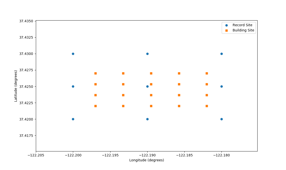
This example is a small-scale regional earthquake risk assessment that performs response simulation and damage/loss estimation for a group of 20 buildings. The buildings are modeled as elastic-perfectly plastic single-degree-of-freedom (SDOF) systems defined by three input model parameters: the weight W, yield strength f_yield, and fundamental period T1. The buildings are distributed in space in a 4x5 grid, within a 3x3 grid of event sites. At each event site, 5 ground motion records of similar intensity are assigned.
4.1.1. Inputs
The example input files can be downloaded here: example_eq.zip. For more information about required input files, refer to Inputs.
Configuration file: The configuration file specifies all simulation settings, including the application types, input file names, units, and types of outputs.
 1{
 2  "Name": "rWHALE_",
 3  "Author": "Adam Zsarnóczay",
 4  "WorkflowType": "Parametric Study",
 5  "runDir": "...",
 6  "localAppDir": "C:/rWHALE/",
 7  "units": {
 8      "force": "kips",
 9      "length": "in",
10      "time": "sec"
11   },
12   "outputs": {
13    "EDP": true,
14    "DM": true,
15    "DV": true,
16    "every_realization": false
17  },
18  "Applications": {
19    "Building": {
20      "Application": "CSV_to_BIM",
21      "ApplicationData": {
22        "Min": "1",
23        "Max": "2",
24        "buildingSourceFile":"input_params.csv"
25      }
26    },
27    "RegionalMapping": {
28      "Application": "NearestNeighborEvents",
29      "ApplicationData": {
30        "filenameEVENTgrid": "records/EventGrid.csv",
31        "samples": 5,
32        "neighbors": 4
33      }
34    },
35    "Events": [{
36      "EventClassification": "Earthquake",
37      "Application": "SimCenterEvent",
38      "ApplicationData": {
39        "pathEventData": "records/"
40      }
41    }],
42    "Modeling": {
43      "Application": "OpenSeesPyInput",
44      "ApplicationData": {
45        "mainScript": "cantilever.py",
46        "modelPath": "model/",
47        "ndm": 3,
48        "dofMap": "1,2,3"
49      }
50    },
51    "EDP": {
52      "Application": "UserDefinedEDP_R",
53      "ApplicationData": {
54        "EDPspecs": "EDP_specs.json"
55      }
56    },
57    "Simulation": {
58       "Application": "OpenSeesPy-Simulation",
59       "ApplicationData": {
60       }
61    },
62    "UQ": {
63       "Application": "Dakota-UQ",
64       "ApplicationData": {
65          "method": "LHS",
66          "samples": 5,
67          "type": "UQ",
68          "concurrency": 1,
69          "keepSamples": true
70       }
71    },
72    "DL": {
73            "Application": "pelicun",
74            "ApplicationData": {
75                "DL_Method": "HAZUS MH EQ",
76                "Realizations": 5,
77                "detailed_results": false,
78                "log_file": true,
79                "coupled_EDP": true,
80                "event_time": "off",
81                "ground_failure": false
82            }
83        }
84    }
85}
Building Application: This example uses the CSV_to_BIM building application. In the configuration file, the Max and Min parameters are set to run the full set of 20 buildings, and the name of the building source file is provided as “input_params.csv”. In the building source file, input parameters for (a) the response simulation (weight
W, yield strengthf_yield, and fundamental periodT1) and for (b) the DL assessment (e.g.,NumberofStories,YearBuilt,OccupancyClass,StructureType,PlanArea,ReplacementCost) are specified.
Building source file:
id |
Latitude |
Longitude |
NumberofStories |
YearBuilt |
OccupancyClass |
StructureType |
PlanArea |
ReplacementCost |
W |
f_yield |
T1 |
|---|---|---|---|---|---|---|---|---|---|---|---|
0 |
37.422 |
-122.182 |
1 |
1957 |
RES1 |
W1 |
1293.253476 |
1 |
55.25 |
118.75 |
0.29375 |
1 |
37.422 |
-122.18575 |
1 |
1927 |
RES1 |
W1 |
2568.835761 |
1 |
86.75 |
148.75 |
0.15625 |
2 |
37.422 |
-122.1895 |
1 |
2020 |
RES1 |
W1 |
1127.07738 |
1 |
114.75 |
123.75 |
0.39375 |
3 |
37.422 |
-122.19325 |
1 |
1951 |
RES1 |
W1 |
2085.809768 |
1 |
107.75 |
126.25 |
0.24375 |
4 |
37.422 |
-122.197 |
1 |
1960 |
RES1 |
W1 |
1481.567067 |
1 |
76.25 |
101.25 |
0.30625 |
5 |
37.42366667 |
-122.182 |
1 |
1986 |
RES1 |
W1 |
1240.719532 |
1 |
90.25 |
116.25 |
0.21875 |
6 |
37.42366667 |
-122.18575 |
1 |
1984 |
RES1 |
W1 |
2437.970509 |
1 |
93.75 |
141.25 |
0.35625 |
7 |
37.42366667 |
-122.1895 |
1 |
1983 |
RES1 |
W1 |
2668.60615 |
1 |
111.25 |
133.75 |
0.36875 |
8 |
37.42366667 |
-122.19325 |
1 |
1957 |
RES1 |
W1 |
1553.47035 |
1 |
104.25 |
108.75 |
0.19375 |
9 |
37.42366667 |
-122.197 |
1 |
1984 |
RES1 |
W1 |
1625.164708 |
1 |
58.75 |
106.25 |
0.23125 |
10 |
37.42533333 |
-122.182 |
1 |
2018 |
RES1 |
W1 |
1787.865419 |
1 |
62.25 |
143.75 |
0.34375 |
11 |
37.42533333 |
-122.18575 |
1 |
2018 |
RES1 |
W1 |
1821.174819 |
1 |
65.75 |
138.75 |
0.20625 |
12 |
37.42533333 |
-122.1895 |
1 |
1930 |
RES1 |
W1 |
1624.532488 |
1 |
69.25 |
146.25 |
0.31875 |
13 |
37.42533333 |
-122.19325 |
1 |
1922 |
RES1 |
W1 |
1134.673241 |
1 |
79.75 |
103.75 |
0.25625 |
14 |
37.42533333 |
-122.197 |
1 |
1947 |
RES1 |
W1 |
1625.097354 |
1 |
51.75 |
128.75 |
0.16875 |
15 |
37.427 |
-122.182 |
1 |
1969 |
RES1 |
W1 |
2289.96328 |
1 |
83.25 |
131.25 |
0.33125 |
16 |
37.427 |
-122.18575 |
1 |
2006 |
RES1 |
W1 |
2288.360712 |
1 |
100.75 |
136.25 |
0.38125 |
17 |
37.427 |
-122.1895 |
1 |
1959 |
RES1 |
W1 |
2291.605647 |
1 |
97.25 |
111.25 |
0.18125 |
18 |
37.427 |
-122.19325 |
1 |
1979 |
RES1 |
W1 |
2770.811412 |
1 |
72.75 |
113.75 |
0.26875 |
19 |
37.427 |
-122.197 |
1 |
1976 |
RES1 |
W1 |
2088.450773 |
1 |
118.25 |
121.25 |
0.28125 |
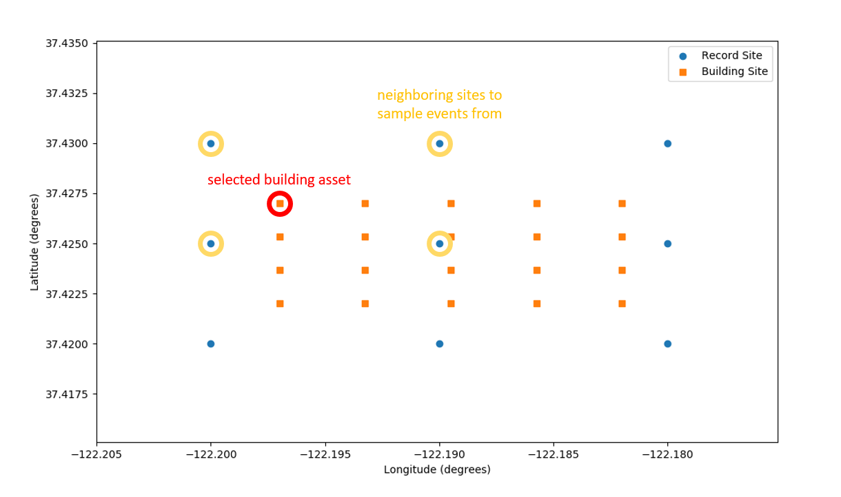
Regional Mapping Application: This example uses the NearestNeighborEvents regional mapping application. From the parameters set in the configuration file, the algorithm is set to randomly select 5 samples of ground motion records from the 4 nearest neighbors for each building asset.
Event Application: This example uses the SimCenterEvents event application. It takes as input the EventGrid.csv, event files with the ground motion intensity measures, and the site files that specify the five ground motions assigned to each event site.
Event grid file:
sta |
lon |
lat |
|---|---|---|
site0.csv |
-122.18 |
37.42 |
site1.csv |
-122.19 |
37.42 |
site2.csv |
-122.2 |
37.42 |
site3.csv |
-122.18 |
37.425 |
site4.csv |
-122.19 |
37.425 |
site5.csv |
-122.2 |
37.425 |
site6.csv |
-122.18 |
37.43 |
site7.csv |
-122.19 |
37.43 |
site8.csv |
-122.2 |
37.43 |
Site file:
GM_file |
factor |
|---|---|
RSN251 |
4.683735054680426 |
RSN564 |
1.2243750794265975 |
RSN692 |
0.8188602253372889 |
RSN626 |
1.252450834874058 |
RSN244 |
4.634837258912294 |
Modeling Application: This example uses the OpenSeesPyInput modeling application. The buildings are modeled as elastic-perfectly plastic single-degree-of-freedom (SDOF) systems defined by three input model parameters: the weight
W, yield strengthf_yield, and fundamental periodT1. Functions are included which record the peak response as EDPs for each of the EDP types specified in the EDP_specs.json file.
Model file:
  1import numpy as np
  2from math import pi, sqrt
  3from openseespy.opensees import *
  4import os
  5
  6
  7''' FUNCTION: build_model ------------------------------------------------------
  8Generates OpenSeesPy model of an elastic-perfectly plastic SDOF system and runs
  9gravity analysis.
 10Inputs: in model_params
 11	W - weight of structure
 12	f_yield - yield stiffness
 13	T1 - fundamental period
 14Outputs:
 15
 16-----------------------------------------------------------------------------'''
 17
 18def build_model(model_params):
 19
 20	G = 386.1
 21	W = model_params["W"]
 22	f_yield = model_params["f_yield"]
 23	T1 = model_params["T1"]
 24	m = W / G
 25	print("m: " + str(m))
 26
 27	# set model dimensions and deg of freedom
 28	model('basic', '-ndm', 3, '-ndf', 6)
 29
 30	# define nodes
 31	base_node_tag = 10000
 32	top_node_tag = 10001
 33	height = 240. # in
 34	node(base_node_tag, 0., 0., 0.)
 35	node(top_node_tag, 0., 0., height)
 36
 37	# define fixities
 38	fix(base_node_tag, 1, 1, 1, 1, 1, 1)
 39	fix(top_node_tag, 0, 0, 0, 1, 1, 1)
 40
 41	# define bilinear (elastic-perfectly plastic) material
 42	material_tag = 100
 43	stiffmat = 110
 44	K = m / (T1/(2*pi))**2
 45	print("K: " + str(K))
 46	uniaxialMaterial('Steel01', material_tag, f_yield, K, 0.0001)
 47	uniaxialMaterial('Elastic', stiffmat, 1.e9)
 48
 49	# define element
 50	element_tag = 1000
 51	element('twoNodeLink', element_tag, base_node_tag, top_node_tag, '-mat', stiffmat, material_tag, material_tag, '-dir', 1, 2, 3, '-orient', 0., 0., 1., 0., 1., 0., '-doRayleigh')
 52
 53	# define mass
 54	mass(top_node_tag, m, m, m, 0., 0., 0.)
 55
 56	# define gravity loads
 57	# W = m * 386.01 # g
 58	timeSeries('Linear', 1)
 59	pattern('Plain', 101, 1)
 60	load(top_node_tag, 0., 0., -W, 0., 0., 0.)
 61
 62	# define damping based on first eigenmode
 63	damp_ratio = 0.05
 64	angular_freq = eigen(1)[0]**0.5
 65	beta_k = 2 * damp_ratio / angular_freq
 66	rayleigh(0., beta_k, 0., 0.)
 67
 68	# run gravity analysis
 69	tol = 1e-8                          # convergence tolerance for test
 70	iter = 100                          # max number of iterations
 71	nstep = 100               		    # apply gravity loads in 10 steps
 72	incr = 1./nstep          			# first load increment
 73
 74	# analysis settings
 75	constraints('Transformation')       # enforce boundary conditions using transformation constraint handler
 76	numberer('RCM')			            # renumbers dof's to minimize band-width (optimization)
 77	system('BandGeneral')		        # stores system of equations as 1D array of size bandwidth x number of unknowns
 78	test('EnergyIncr', tol, iter, 0)    # tests for convergence using dot product of solution vector and norm of right-hand side of matrix equation
 79	algorithm('Newton')                 # use Newton's solution algorithm: updates tangent stiffness at every iteration
 80	integrator('LoadControl', incr)     # determine the next time step for an analysis # apply gravity in 10 steps
 81	analysis('Static')		            # define type of analysis, static or transient
 82	analyze(nstep)	          			# perform gravity analysis
 83
 84	# after gravity analysis, change time and tolerance for the dynamic analysis
 85	loadConst('-time', 0.0)
 86
 87
 88
 89
 90
 91
 92# FUNCTION: PeakDriftRecorder --------------------------------------------------
 93# saves envelope of interstory drift ratio for each story at one analysis step
 94# ------------------------------------------------------------------------------
 95
 96def PeakDriftRecorder(EDP_specs, envDict):
 97    # inputs:
 98    # EDP_specs = dictionary of EDP type, location, direction
 99    # envDict = dictionary of envelope values
100
101
102    for loc in EDP_specs['PID']:
103        pos = 0
104        for dof in EDP_specs['PID'][loc]:
105            storynodes = [int(x) for x in EDP_specs['PID'][loc][dof]]
106            # print("computing drifts for nodes: {}".format(storynodes))
107            story_height = nodeCoord(storynodes[1],3) - nodeCoord(storynodes[0],3)
108            # compute drift
109            topDisp = nodeDisp(storynodes[1],dof)
110            botDisp = nodeDisp(storynodes[0],dof)
111            new_drift = abs((topDisp-botDisp)/story_height)
112            # update dictionary
113            curr_drift = envDict['PID'][loc][pos]
114            new_max = max(new_drift, curr_drift)
115            envDict['PID'][loc][pos] = new_max
116            pos += 1
117
118    return envDict
119
120
121
122# FUNCTION: AccelHistoryRecorder -----------------------------------------------
123# saves time history of relative floor acceleration for each story at one analysis step
124# ------------------------------------------------------------------------------
125
126def AccelHistoryRecorder(EDP_specs, histDict, count):
127    # inputs:
128    # histDict = dictionary of time histories
129    # recorderNodes = list of nodes where EDP is recorded
130    # count = current count in the time history
131
132    for loc in EDP_specs['PFA']:
133        for dof in EDP_specs['PFA'][loc]:
134            storynode = int(EDP_specs['PFA'][loc][dof][0])
135            # obtain acceleration
136            new_acc = nodeAccel(storynode, dof)
137            histDict['accel'][loc][dof][count] = new_acc
138
139
140    return histDict
141
142
143
144# FUNCTION: RunDynamicAnalysis -------------------------------------------------
145# performs dynamic analysis and records EDPs in dictionary
146# ------------------------------------------------------------------------------
147
148def RunDynamicAnalysis(tol,iter,dt,driftLimit,EDP_specs,subSteps,GMX,GMZ):
149    # inputs:
150    # tol = tolerance criteria to check for convergence
151    # iter = max number of iterations to check
152    # dt = time increment for analysis
153    # driftLimit = percent interstory drift limit indicating collapse
154    # recorderNodes = vector of node labels used to check global drifts and record EDPs
155    # subSteps = number of subdivisions in cases of ill convergence
156    # GMX = list of GM acceleration ordinates in X direction
157    # GMZ = list of GM acceleration ordinates in Z direction
158
159    # pad shorter record with zeros (free vibration) such that two horizontal records are the same length
160    nsteps = max(len(GMX),len(GMZ))
161    if len(GMX) < nsteps:
162        diff = nsteps - len(GMX)
163        GMX.extend(np.zeros(diff))
164    if len(GMZ) < nsteps:
165        diff = nsteps - len(GMZ)
166        GMZ.extend(np.zeros(diff))
167
168
169    # generate time array from recording
170    time_record = np.linspace(0,nsteps*dt,num=nsteps,endpoint=False)
171
172    # initialize dictionary of envelope EDPs
173    envelopeDict = {}
174    for edp in EDP_specs:
175        envelopeDict[edp] = {}
176        for loc in EDP_specs[edp]:
177            numdof = len(EDP_specs[edp][loc])
178            envelopeDict[edp][loc] = np.zeros(numdof).tolist()
179
180    print(envelopeDict)
181
182    # initialize dictionary of time history EDPs
183    historyDict = {'accel':{}}
184    time_analysis = np.zeros(nsteps*5)
185    for loc in EDP_specs['PFA']:
186        historyDict['accel'][loc] = {}
187        for dof in EDP_specs['PFA'][loc]:
188            historyDict['accel'][loc][dof] = np.zeros(nsteps*5)
189
190    # number of diaphragm levels
191    levels = len(EDP_specs['PFA'])
192    CODnodes = []
193    for loc in EDP_specs['PFA']:
194        CODnodes.append(int(EDP_specs['PFA'][loc][1][0]))
195
196    print(CODnodes)
197
198
199    constraints('Transformation')            # handles boundary conditions based on transformation equation method
200    numberer('RCM')                          # renumber dof's to minimize band-width (optimization)
201    system('UmfPack')                        # constructs sparse system of equations using UmfPack solver
202    test('NormDispIncr',tol,iter)            # tests for convergence using norm of left-hand side of matrix equation
203    algorithm('NewtonLineSearch')            # use Newton's solution algorithm: updates tangent stiffness at every iteration
204    integrator('Newmark', 0.5, 0.25)         # Newmark average acceleration method for numerical integration
205    analysis('Transient')                    # define type of analysis: time-dependent
206
207    # initialize variables
208    maxDiv = 1024
209    minDiv = subSteps
210    step = 0
211    ok = 0
212    breaker = 0
213    maxDrift = 0
214    count = 0
215
216    while step<nsteps and ok==0 and breaker==0:
217        step = step + 1  # take 1 step
218        ok = 2
219        div = minDiv
220        length = maxDiv
221        while div<=maxDiv and length>0 and breaker==0:
222            stepSize = dt/div
223            ok = analyze(1,stepSize)               # perform analysis for one increment; will return 0 if no convergence issues
224            if ok==0:
225                count = count + 1
226                length = length - maxDiv/div
227                # check if drift limits are satisfied
228                level = 1
229                while level < levels:
230                    story_height = nodeCoord(CODnodes[level],3)-nodeCoord(CODnodes[level-1],3)
231                    # check X direction drifts (direction 1)
232                    topDisp = nodeDisp(CODnodes[level],1)
233                    botDisp = nodeDisp(CODnodes[level-1],1)
234                    deltaDisp = abs(topDisp-botDisp)
235                    drift = deltaDisp/story_height
236                    if drift >= driftLimit:
237                        breaker = 1
238                    # check Y direction drifts (direction 2)
239                    topDisp = nodeDisp(CODnodes[level],2)
240                    botDisp = nodeDisp(CODnodes[level-1],2)
241                    deltaDisp = abs(topDisp-botDisp)
242                    drift = deltaDisp/story_height
243                    if drift >= driftLimit:
244                        breaker = 1
245                    # move on to check next level
246                    level = level + 1
247                # save parameter values in recording dictionaries at every step
248                time_analysis[count] = time_analysis[count-1]+stepSize
249                envelopeDict = PeakDriftRecorder(EDP_specs, envelopeDict)
250                historyDict = AccelHistoryRecorder(EDP_specs, historyDict, count)
251            else: # if ok != 0
252                div = div*2
253                print("Number of increments increased to ",str(div))
254    # end analysis once drift limit has been reached
255    if breaker == 1:
256        ok = 1
257        print("Collapse drift has been reached")
258
259    print("Number of analysis steps completed: {}".format(count))
260
261    # remove extra zeros from time history
262    time_analysis = time_analysis[1:count+1]
263    historyDict['time'] = time_analysis.tolist()
264
265    # remove extra zeros from accel time history, add GM to obtain absolute acceleration, and record envelope value
266    GMX_interp = np.interp(time_analysis, time_record, GMX)
267    GMZ_interp = np.interp(time_analysis, time_record, GMZ)
268    for level in range(0,levels):
269        # X direction
270        historyDict['accel'][level][1] = historyDict['accel'][level][1][1:count+1]
271        historyDict['accel'][level][1] = np.asarray(historyDict['accel'][level][1]) + GMX_interp
272        envelopeDict['PFA'][level][0] = max(abs(historyDict['accel'][level][1]))
273        # Z direction
274        historyDict['accel'][level][2] = historyDict['accel'][level][2][1:count+1]
275        historyDict['accel'][level][2] = np.asarray(historyDict['accel'][level][2]) + GMZ_interp
276        envelopeDict['PFA'][level][1] = max(abs(historyDict['accel'][level][2]))
277
278
279    return envelopeDict
280
281
282
283# MAIN: run_analysis -----------------------------------------------------------
284# runs dynamic analysis for single event and returns dictionary of envelope EDPs
285# ------------------------------------------------------------------------------
286
287def run_analysis(GM_dt, GM_npts, TS_List, EDP_specs):
288    # inputs:
289    # GM_dt = time step of GM record
290    # GM_npts = number of steps in GM record
291    # TS_List = 1x2 list where first component is a list of GMX acceleration points, second component is a list of GMZ acceleration points (scaled and multipled by G)
292    GMX_points = TS_List[0]
293    GMZ_points = TS_List[1]
294
295    # print(EDP_specs)
296
297    wipeAnalysis()
298
299
300    # define parameters for dynamic analysis
301    driftLimit = 0.20   # %
302    toler = 1.e-08
303    maxiter = 30
304    subSteps = 2
305
306    envdata = RunDynamicAnalysis(toler,maxiter,GM_dt,driftLimit,EDP_specs,subSteps,GMX_points,GMZ_points)
307    print(envdata)
308
309    return envdata
EDP Application: This example uses the UserDefinedEDP EDP application. Custom EDPs are specified in the EDP specifications file. The EDP types are peak interstory drift (PID) and peak floor acceleration (PFA), recorded at the base and top node of the structural model in two horizontal directions (1,2).
EDP specifications file:
 1{
 2    "locations": {
 3        "0": [
 4            10000,
 5            10001
 6        ]
 7    },
 8    "EDP_types": {
 9        "PID": {
10            "0": [
11                1,
12                2
13            ]
14        },
15        "PFA": {
16            "0": [
17                1,
18                2
19            ]
20        }
21    }
22}
Simulation Application: This example uses the OpenSeesPySimulation simulation application, which corresponds to the OpenSeesPyInput modeling application. It reads the
build_modelandrun_analysisfunctions from the model file to perform the response simulation.UQ Application: This example uses the Dakota-UQ UQ application to run the response simulation. In the configuration file, the number of samples specified for the UQ application should match the number of ground motion samples per building asset specified for the RegionalMapping application.
DL Application: This example uses the pelicun DL application. From the building source file, since the DL method selected is “HAZUS MH EQ”, damage/loss estimation is performed using the HAZUS loss assessment method based on earthquake EDPs produced from the response simulation.
4.1.2. Run Workflow
The workflow can be executed by uploading the appropriate files to DesignSafe, or by running the example on your local desktop, using the following initialization command in the terminal:
python "C:/rWHALE/applications/Workflow/R2D_workflow.py" "C:/rWHALE/cantilever_example/rWHALE_config_eq.json" --registry "C:/rWHALE/applications/Workflow/WorkflowApplications.json" --referenceDir "C:/rWHALE/cantilever_example/input_data/" -w "C:/rWHALE/cantilever_example/results"
This command locates the backend applications in the folder “applications” and the input files in a directory “cantilever_example”. Please ensure that the paths in the command appropriately identify the locations of the files in your directory.
applications
cantilever_example
├── rWHALE_config_eq.json              # configuration file
└── input_data
    ├── model
        ├── cantilever.py           # model file
    ├── records
        ├── EventGrid.csv           # event grid file
        ├── RSN30.json              # event IM files
        ├── RSN63.json
        .
        .
        .
        ├── site0.csv               # site files
        ├── site1.csv
        .
        .
        .
        └── site8.csv
    ├── EDPspecs.json               # EDP specifications file
    └── input_params.csv            # building source file
4.1.3. Outputs
The example output files can be downloaded here: output_data_eq.zip. For more information about the output files produced, refer to Outputs.
EDP_1-19.csv: reports statistics on the EDP results from simulating 5 ground motions for each building asset. The statistics reported are the median and lognormal standard deviation of peak interstory drift (PID) and peak floor acceleration (PFA) in two directions.
type |
PFA |
PFA |
PFA |
PFA |
PFA |
PFA |
PFA |
PFA |
PID |
PID |
PID |
PID |
|---|---|---|---|---|---|---|---|---|---|---|---|---|
loc |
0 |
0 |
0 |
0 |
1 |
1 |
1 |
1 |
1 |
1 |
1 |
1 |
dir |
1 |
1 |
2 |
2 |
1 |
1 |
2 |
2 |
1 |
1 |
2 |
2 |
stat |
median |
beta |
median |
beta |
median |
beta |
median |
beta |
median |
beta |
median |
beta |
1 |
141.097 |
0.199749331936861 |
136.972 |
0.26159704860592325 |
412.267 |
0.3689067092818622 |
271.872 |
0.4675055669073214 |
0.00105633 |
0.4186167860756997 |
0.0006980389999999999 |
0.5784022941837268 |
2 |
131.247 |
0.4175448180418805 |
155.204 |
0.20283668507914568 |
176.59 |
0.4337498687956456 |
157.04 |
0.2691536257751124 |
0.00287297 |
0.4355512490436657 |
0.00255504 |
0.2712436832366108 |
3 |
144.195 |
0.3556909851130682 |
138.769 |
0.14200186407081142 |
446.805 |
0.37406788320556 |
317.6 |
0.232094515864188 |
0.00278474 |
0.42430956257276864 |
0.00198152 |
0.3651330947055237 |
4 |
141.43 |
0.2621121131463965 |
149.726 |
0.13936603018873167 |
252.456 |
0.20223535336029075 |
358.745 |
0.4682999285137096 |
0.00248399 |
0.20078394541079414 |
0.00353105 |
0.4664649292002271 |
5 |
127.76799999999999 |
0.1933699100399082 |
162.64700000000005 |
0.22228311460245634 |
373.093 |
0.2695036478790295 |
361.592 |
0.21513981161420967 |
0.0018780000000000001 |
0.2699071050235337 |
0.00181748 |
0.2155059270390112 |
6 |
182.01400000000004 |
0.1878891925155105 |
160.911 |
0.19737203237767328 |
292.335 |
0.48771266468706703 |
292.813 |
0.2930718377890685 |
0.00389908 |
0.4877100061602449 |
0.00390263 |
0.2931719410768729 |
7 |
130.996 |
0.3926228335954007 |
145.494 |
0.09229922720084753 |
267.488 |
0.237269603979 |
146.707 |
0.3405650974061709 |
0.00382051 |
0.2371602524305522 |
0.00209569 |
0.3414405710280442 |
8 |
130.996 |
0.3926228335954007 |
145.494 |
0.09229922720084753 |
416.75300000000004 |
0.12180918060252133 |
417.148 |
0.07443597424038638 |
0.00205192 |
0.3104238725586141 |
0.00182858 |
0.13467088219923146 |
9 |
143.016 |
0.24358377366199915 |
163.14200000000002 |
0.2019342858851748 |
405.908 |
0.35204871925623343 |
322.71 |
0.08340885973141009 |
0.00227816 |
0.3537066848027953 |
0.00181325 |
0.083987554229959 |
10 |
183.49 |
0.18755333115184367 |
160.376 |
0.13276066086178542 |
488.46 |
0.23272021112520425 |
346.295 |
0.38094421218731933 |
0.00606391 |
0.2332570737380188 |
0.00429183 |
0.3818933891243802 |
11 |
146.18 |
0.18278485835299355 |
160.911 |
0.1991058705931532 |
331.755 |
0.2799965748805636 |
484.579 |
0.32562150845640137 |
0.0014824999999999999 |
0.2803097978527769 |
0.0021631 |
0.3249379345839239 |
12 |
130.996 |
0.3926228335954007 |
145.494 |
0.09229922720084753 |
254.428 |
0.28072218931094045 |
288.997 |
0.3930704970844931 |
0.00271677 |
0.2812514879339413 |
0.0030816 |
0.3928937764199453 |
13 |
143.016 |
0.3786819120652951 |
175.497 |
0.12506807756500646 |
289.259 |
0.12209314196371647 |
311.926 |
0.2268268415312083 |
0.00199303 |
0.12220673894617105 |
0.00215043 |
0.2271012433659633 |
14 |
143.016 |
0.3895371771421967 |
131.827 |
0.2150120977551468 |
425.28600000000006 |
0.18182010821614525 |
473.92900000000003 |
0.1144372496639498 |
0.0012720000000000001 |
0.1819342336642664 |
0.00141906 |
0.11431467535648035 |
15 |
182.01400000000004 |
0.3608990379206519 |
147.194 |
0.2253981063223195 |
389.17800000000005 |
0.3543220031783357 |
428.847 |
0.3687617252701749 |
0.00448564 |
0.3545767941681689 |
0.00494268 |
0.3692013703541936 |
16 |
157.774 |
0.3836750491797111 |
130.084 |
0.19764143187735794 |
287.992 |
0.5030060338225658 |
378.276 |
0.4394897070740103 |
0.00439757 |
0.5081468202869077 |
0.005776399999999999 |
0.43938961960039613 |
17 |
131.71 |
0.3920062442871513 |
150.631 |
0.09242281539618902 |
455.541 |
0.13776975495264546 |
454.36 |
0.2490103895868422 |
0.00176016 |
0.2861092987848653 |
0.00161805 |
0.26566745390451 |
18 |
143.016 |
0.4079243417920144 |
160.911 |
0.14065793137491145 |
297.425 |
0.22852660788272866 |
307.39 |
0.25192434465967034 |
0.00225423 |
0.2287664511405949 |
0.00233144 |
0.2520961518809855 |
19 |
137.914 |
0.4224669047258293 |
131.827 |
0.2054938432485909 |
249.41099999999997 |
0.2679721569521585 |
409.027 |
0.2668373210824858 |
0.0020721 |
0.28311021269960546 |
0.00360748 |
0.31569408537266186 |
DM_1-19.csv: reports collapse probability and damage state probability for each building asset.
Collapse |
DS likelihood |
DS likelihood |
DS likelihood |
DS likelihood |
DS likelihood |
DS likelihood |
DS likelihood |
DS likelihood |
DS likelihood |
DS likelihood |
DS likelihood |
DS likelihood |
DS likelihood |
DS likelihood |
DS likelihood |
DS likelihood |
DS likelihood |
DS likelihood |
DS likelihood |
DS likelihood |
DS likelihood |
|
|---|---|---|---|---|---|---|---|---|---|---|---|---|---|---|---|---|---|---|---|---|---|---|
comp_type |
probability |
S |
S |
S |
S |
S |
S |
NS |
NS |
NS |
NS |
NS |
NSA |
NSA |
NSA |
NSA |
NSA |
NSD |
NSD |
NSD |
NSD |
NSD |
DSG_DS |
0 |
1_1 |
2_1 |
3_1 |
4_1 |
4_2 |
0 |
1_1 |
2_1 |
3_1 |
4_1 |
0 |
1_1 |
2_1 |
3_1 |
4_1 |
0 |
1_1 |
2_1 |
3_1 |
4_1 |
|
1 |
0.0 |
1.0 |
0.0 |
0.0 |
0.0 |
0.0 |
0.0 |
0.0 |
0.4 |
0.2 |
0.2 |
0.2 |
0.0 |
0.4 |
0.2 |
0.2 |
0.2 |
1.0 |
0.0 |
0.0 |
0.0 |
0.0 |
2 |
0.0 |
0.6 |
0.4 |
0.0 |
0.0 |
0.0 |
0.0 |
0.2 |
0.20000000000000007 |
0.4 |
0.0 |
0.2 |
0.2 |
0.20000000000000007 |
0.4 |
0.0 |
0.2 |
0.8 |
0.2 |
0.0 |
0.0 |
0.0 |
3 |
0.0 |
0.4 |
0.6 |
0.0 |
0.0 |
0.0 |
0.0 |
0.0 |
0.2 |
0.4 |
0.0 |
0.4 |
0.0 |
0.2 |
0.4 |
0.0 |
0.4 |
0.6 |
0.4 |
0.0 |
0.0 |
0.0 |
4 |
0.0 |
0.4 |
0.6 |
0.0 |
0.0 |
0.0 |
0.0 |
0.0 |
0.4 |
0.2 |
0.2 |
0.2 |
0.0 |
0.4 |
0.2 |
0.2 |
0.2 |
0.4 |
0.4 |
0.2 |
0.0 |
0.0 |
5 |
0.0 |
1.0 |
0.0 |
0.0 |
0.0 |
0.0 |
0.0 |
0.0 |
0.4 |
0.0 |
0.4 |
0.2 |
0.0 |
0.4 |
0.0 |
0.4 |
0.2 |
0.8 |
0.2 |
0.0 |
0.0 |
0.0 |
6 |
0.0 |
0.4 |
0.6 |
0.0 |
0.0 |
0.0 |
0.0 |
0.2 |
0.20000000000000007 |
0.6 |
0.0 |
0.0 |
0.2 |
0.20000000000000007 |
0.6 |
0.0 |
0.0 |
0.6 |
0.2 |
0.2 |
0.0 |
0.0 |
7 |
0.0 |
0.4 |
0.6 |
0.0 |
0.0 |
0.0 |
0.0 |
0.0 |
0.4 |
0.2 |
0.4 |
0.0 |
0.0 |
0.4 |
0.2 |
0.4 |
0.0 |
0.2 |
0.8 |
0.0 |
0.0 |
0.0 |
8 |
0.0 |
1.0 |
0.0 |
0.0 |
0.0 |
0.0 |
0.0 |
0.0 |
0.0 |
0.2 |
0.6000000000000001 |
0.2 |
0.0 |
0.0 |
0.2 |
0.6000000000000001 |
0.2 |
0.8 |
0.2 |
0.0 |
0.0 |
0.0 |
9 |
0.0 |
0.8 |
0.2 |
0.0 |
0.0 |
0.0 |
0.0 |
0.0 |
0.2 |
0.8 |
0.0 |
0.0 |
0.0 |
0.2 |
0.8 |
0.0 |
0.0 |
0.4 |
0.6 |
0.0 |
0.0 |
0.0 |
10 |
0.0 |
0.6 |
0.4 |
0.0 |
0.0 |
0.0 |
0.0 |
0.0 |
0.0 |
0.4 |
0.2 |
0.4 |
0.0 |
0.0 |
0.4 |
0.2 |
0.4 |
0.6 |
0.2 |
0.2 |
0.0 |
0.0 |
11 |
0.0 |
1.0 |
0.0 |
0.0 |
0.0 |
0.0 |
0.0 |
0.0 |
0.2 |
0.4 |
0.4 |
0.0 |
0.0 |
0.2 |
0.4 |
0.4 |
0.0 |
1.0 |
0.0 |
0.0 |
0.0 |
0.0 |
12 |
0.0 |
1.0 |
0.0 |
0.0 |
0.0 |
0.0 |
0.0 |
0.0 |
0.0 |
0.6 |
0.4 |
0.0 |
0.0 |
0.0 |
0.6 |
0.4 |
0.0 |
0.6 |
0.4 |
0.0 |
0.0 |
0.0 |
13 |
0.0 |
0.8 |
0.2 |
0.0 |
0.0 |
0.0 |
0.0 |
0.0 |
0.6 |
0.4 |
0.0 |
0.0 |
0.0 |
0.6 |
0.4 |
0.0 |
0.0 |
1.0 |
0.0 |
0.0 |
0.0 |
0.0 |
14 |
0.0 |
0.8 |
0.2 |
0.0 |
0.0 |
0.0 |
0.0 |
0.0 |
0.0 |
0.2 |
0.4 |
0.4 |
0.0 |
0.0 |
0.2 |
0.4 |
0.4 |
1.0 |
0.0 |
0.0 |
0.0 |
0.0 |
15 |
0.0 |
0.4 |
0.6 |
0.0 |
0.0 |
0.0 |
0.0 |
0.0 |
0.0 |
0.6 |
0.2 |
0.2 |
0.0 |
0.0 |
0.6 |
0.2 |
0.2 |
0.6 |
0.2 |
0.2 |
0.0 |
0.0 |
16 |
0.0 |
0.4 |
0.6 |
0.0 |
0.0 |
0.0 |
0.0 |
0.0 |
0.0 |
0.4 |
0.6 |
0.0 |
0.0 |
0.0 |
0.4 |
0.6 |
0.0 |
0.0 |
0.6 |
0.4 |
0.0 |
0.0 |
17 |
0.0 |
1.0 |
0.0 |
0.0 |
0.0 |
0.0 |
0.0 |
0.0 |
0.0 |
0.0 |
0.6 |
0.4 |
0.0 |
0.0 |
0.0 |
0.6 |
0.4 |
1.0 |
0.0 |
0.0 |
0.0 |
0.0 |
18 |
0.0 |
0.6 |
0.4 |
0.0 |
0.0 |
0.0 |
0.0 |
0.0 |
0.4 |
0.2 |
0.2 |
0.2 |
0.2 |
0.20000000000000007 |
0.2 |
0.2 |
0.2 |
0.4 |
0.6 |
0.0 |
0.0 |
0.0 |
19 |
0.0 |
0.8 |
0.2 |
0.0 |
0.0 |
0.0 |
0.0 |
0.0 |
0.6 |
0.2 |
0.2 |
0.0 |
0.2 |
0.4 |
0.2 |
0.2 |
0.0 |
0.6 |
0.4 |
0.0 |
0.0 |
0.0 |
DV_1-19.csv: reports decision variable estimates (repair cost, repair time, injuries) for each building asset.
DV |
Repair Cost |
Repair Cost |
Repair Cost |
Repair Cost |
Repair Cost |
Repair Impractical |
Repair Cost |
Repair Cost |
Repair Cost |
Repair Cost |
Repair Cost |
Repair Cost |
Repair Cost |
Repair Cost |
Repair Cost |
Repair Cost |
Repair Cost |
Repair Cost |
Repair Cost |
Repair Cost |
Repair Cost |
Repair Cost |
Repair Cost |
Repair Cost |
Repair Cost |
Repair Cost |
Repair Cost |
Repair Time |
Repair Time |
Repair Time |
Repair Time |
Repair Time |
Injuries |
Injuries |
Injuries |
Injuries |
Injuries |
Injuries |
Injuries |
Injuries |
Injuries |
Injuries |
Injuries |
Injuries |
Injuries |
Injuries |
Injuries |
Injuries |
Injuries |
Injuries |
Injuries |
Injuries |
|---|---|---|---|---|---|---|---|---|---|---|---|---|---|---|---|---|---|---|---|---|---|---|---|---|---|---|---|---|---|---|---|---|---|---|---|---|---|---|---|---|---|---|---|---|---|---|---|---|---|---|---|---|
comp_type |
aggregate |
aggregate |
aggregate |
aggregate |
aggregate |
probability |
S |
S |
S |
S |
S |
S |
NS |
NS |
NS |
NS |
NS |
NSA |
NSA |
NSA |
NSA |
NSA |
NSD |
NSD |
NSD |
NSD |
NSD |
sev1 |
sev1 |
sev1 |
sev1 |
sev1 |
sev2 |
sev2 |
sev2 |
sev2 |
sev2 |
sev3 |
sev3 |
sev3 |
sev3 |
sev3 |
sev4 |
sev4 |
sev4 |
sev4 |
sev4 |
|||||
DSG_DS |
aggregate |
1_1 |
2_1 |
3_1 |
4_1 |
4_2 |
aggregate |
1_1 |
2_1 |
3_1 |
4_1 |
aggregate |
1_1 |
2_1 |
3_1 |
4_1 |
aggregate |
1_1 |
2_1 |
3_1 |
4_1 |
aggregate |
aggregate |
aggregate |
aggregate |
aggregate |
aggregate |
aggregate |
aggregate |
aggregate |
aggregate |
aggregate |
aggregate |
aggregate |
aggregate |
aggregate |
aggregate |
aggregate |
aggregate |
aggregate |
aggregate |
aggregate |
aggregate |
aggregate |
aggregate |
aggregate |
||||||
stat |
mean |
std |
10% |
median |
90% |
mean |
mean |
mean |
mean |
mean |
mean |
mean |
mean |
mean |
mean |
mean |
mean |
mean |
mean |
mean |
mean |
mean |
mean |
mean |
mean |
mean |
mean |
std |
10% |
median |
90% |
mean |
std |
10% |
median |
90% |
mean |
std |
10% |
median |
90% |
mean |
std |
10% |
median |
90% |
mean |
std |
10% |
median |
90% |
|
1 |
0.0766 |
0.098587220267132 |
0.005 |
0.027000000000000003 |
0.1916 |
0.0 |
0.0 |
0.0766 |
0.005 |
0.027000000000000003 |
0.08 |
0.266 |
0.0766 |
0.005 |
0.027000000000000003 |
0.08 |
0.266 |
0.0 |
0.0 |
0.0 |
0.0 |
0.0 |
0.0 |
0.0 |
0.0 |
0.0 |
0.0 |
0.0 |
0.0 |
0.0 |
0.0 |
0.0 |
0.0 |
0.0 |
0.0 |
0.0 |
0.0 |
0.0 |
0.0 |
0.0 |
0.0 |
0.0 |
0.0 |
|||||||||
2 |
0.06790000000000003 |
0.10501438591926347 |
0.0034500000000000004 |
0.027000000000000003 |
0.17692500000000005 |
0.0 |
0.00145 |
0.003625 |
0.06645000000000001 |
0.005 |
0.027000000000000003 |
0.27325 |
0.06500000000000003 |
0.005 |
0.027000000000000003 |
0.266 |
0.00145 |
0.007249999999999999 |
0.58 |
0.7103520254071216 |
0.0 |
0.0 |
1.45 |
0.000145 |
0.00017758800635178038 |
0.0 |
0.0 |
0.0003625 |
0.0 |
0.0 |
0.0 |
0.0 |
0.0 |
0.0 |
0.0 |
0.0 |
0.0 |
0.0 |
0.0 |
0.0 |
0.0 |
0.0 |
0.0 |
|||||||||
3 |
0.12327500000000002 |
0.12416358665083738 |
0.015975000000000003 |
0.030625000000000006 |
0.27542500000000003 |
0.0 |
0.002175 |
0.003625 |
0.1211 |
0.005 |
0.027000000000000003 |
0.27325 |
0.1182 |
0.005 |
0.027000000000000003 |
0.266 |
0.0029 |
0.007249999999999999 |
0.8699999999999999 |
0.7103520254071216 |
0.0 |
1.45 |
1.45 |
0.0002175 |
0.00017758800635178038 |
0.0 |
0.0003625 |
0.0003625 |
0.0 |
0.0 |
0.0 |
0.0 |
0.0 |
0.0 |
0.0 |
0.0 |
0.0 |
0.0 |
0.0 |
0.0 |
0.0 |
0.0 |
0.0 |
|||||||||
4 |
0.0911 |
0.10353626780022544 |
0.010075 |
0.030625000000000006 |
0.2177 |
0.0 |
0.0029 |
0.004833333333333333 |
0.0882 |
0.008625 |
0.027000000000000003 |
0.1235 |
0.27325 |
0.07660000000000003 |
0.005 |
0.027000000000000003 |
0.08 |
0.266 |
0.0116 |
0.007249999999999999 |
0.0435 |
1.16 |
1.085080642164443 |
0.0 |
1.45 |
2.3200000000000003 |
0.00029 |
0.00027127016054111073 |
0.0 |
0.0003625 |
0.00058 |
0.0 |
0.0 |
0.0 |
0.0 |
0.0 |
0.0 |
0.0 |
0.0 |
0.0 |
0.0 |
0.0 |
0.0 |
0.0 |
0.0 |
0.0 |
||||||
5 |
0.08865 |
0.09427295476434376 |
0.0079 |
0.08 |
0.1916 |
0.0 |
0.0 |
0.08865 |
0.008625 |
0.08 |
0.266 |
0.08720000000000001 |
0.005 |
0.08 |
0.266 |
0.00145 |
0.007249999999999999 |
0.0 |
0.0 |
0.0 |
0.0 |
0.0 |
0.0 |
0.0 |
0.0 |
0.0 |
0.0 |
0.0 |
0.0 |
0.0 |
0.0 |
0.0 |
0.0 |
0.0 |
0.0 |
0.0 |
0.0 |
0.0 |
0.0 |
0.0 |
0.0 |
0.0 |
||||||||||
6 |
0.036050000000000006 |
0.032783246483531814 |
0.0107 |
0.027000000000000003 |
0.07195000000000001 |
0.0 |
0.0029 |
0.004833333333333333 |
0.03315 |
0.01225 |
0.051166666666666666 |
0.0172 |
0.005 |
0.02700000000000001 |
0.01595 |
0.007249999999999999 |
0.0725 |
1.16 |
1.085080642164443 |
0.0 |
1.45 |
2.3200000000000003 |
0.00029 |
0.00027127016054111073 |
0.0 |
0.0003625 |
0.00058 |
0.0 |
0.0 |
0.0 |
0.0 |
0.0 |
0.0 |
0.0 |
0.0 |
0.0 |
0.0 |
0.0 |
0.0 |
0.0 |
0.0 |
0.0 |
||||||||||
7 |
0.050275 |
0.04010723126818904 |
0.010075 |
0.03425 |
0.09885 |
0.0 |
0.003625 |
0.006041666666666666 |
0.04665 |
0.008625 |
0.03425 |
0.090875 |
0.0394 |
0.005 |
0.027000000000000003 |
0.08 |
0.007249999999999999 |
0.0090625 |
1.45 |
1.2969194269498778 |
0.0 |
1.45 |
2.9 |
0.0003625 |
0.0003242298567374695 |
0.0 |
0.0003625 |
0.000725 |
0.0 |
0.0 |
0.0 |
0.0 |
0.0 |
0.0 |
0.0 |
0.0 |
0.0 |
0.0 |
0.0 |
0.0 |
0.0 |
0.0 |
0.0 |
|||||||||
8 |
0.10805 |
0.08188229356826786 |
0.048200000000000014 |
0.08 |
0.1945 |
0.0 |
0.0 |
0.10805 |
0.027000000000000003 |
0.08241666666666668 |
0.266 |
0.1066 |
0.027000000000000003 |
0.08 |
0.266 |
0.00145 |
0.007249999999999999 |
0.0 |
0.0 |
0.0 |
0.0 |
0.0 |
0.0 |
0.0 |
0.0 |
0.0 |
0.0 |
0.0 |
0.0 |
0.0 |
0.0 |
0.0 |
0.0 |
0.0 |
0.0 |
0.0 |
0.0 |
0.0 |
0.0 |
0.0 |
0.0 |
0.0 |
||||||||||
9 |
0.029125000000000005 |
0.01298075498574717 |
0.013800000000000005 |
0.03425 |
0.04005 |
0.0 |
0.000725 |
0.003625 |
0.0284 |
0.005 |
0.03425 |
0.0226 |
0.005 |
0.027000000000000003 |
0.0058 |
0.009666666666666664 |
0.29 |
0.5800000000000001 |
0.0 |
0.0 |
0.8700000000000001 |
7.25e-05 |
0.000145 |
0.0 |
0.0 |
0.00021750000000000006 |
0.0 |
0.0 |
0.0 |
0.0 |
0.0 |
0.0 |
0.0 |
0.0 |
0.0 |
0.0 |
0.0 |
0.0 |
0.0 |
0.0 |
0.0 |
|||||||||||
10 |
0.151325 |
0.12904455625868144 |
0.032075000000000006 |
0.08 |
0.3124 |
0.0 |
0.002175 |
0.0054375 |
0.14915 |
0.027000000000000003 |
0.08 |
0.305875 |
0.1332 |
0.027000000000000003 |
0.08 |
0.266 |
0.01595 |
0.007249999999999999 |
0.0725 |
0.8699999999999999 |
1.16 |
0.0 |
0.0 |
2.3200000000000003 |
0.0002175 |
0.00028999999999999995 |
0.0 |
0.0 |
0.00058 |
0.0 |
0.0 |
0.0 |
0.0 |
0.0 |
0.0 |
0.0 |
0.0 |
0.0 |
0.0 |
0.0 |
0.0 |
0.0 |
0.0 |
0.0 |
||||||||
11 |
0.0438 |
0.030629397643440526 |
0.013800000000000005 |
0.027000000000000003 |
0.08 |
0.0 |
0.0 |
0.0438 |
0.005 |
0.027000000000000003 |
0.08 |
0.0438 |
0.005 |
0.027000000000000003 |
0.08 |
0.0 |
0.0 |
0.0 |
0.0 |
0.0 |
0.0 |
0.0 |
0.0 |
0.0 |
0.0 |
0.0 |
0.0 |
0.0 |
0.0 |
0.0 |
0.0 |
0.0 |
0.0 |
0.0 |
0.0 |
0.0 |
0.0 |
0.0 |
0.0 |
0.0 |
0.0 |
|||||||||||
12 |
0.054000000000000006 |
0.028037474921968283 |
0.027000000000000003 |
0.0415 |
0.0887 |
0.0 |
0.0 |
0.054000000000000006 |
0.03183333333333333 |
0.08725 |
0.0482 |
0.02700000000000001 |
0.08 |
0.0058 |
0.0145 |
0.0 |
0.0 |
0.0 |
0.0 |
0.0 |
0.0 |
0.0 |
0.0 |
0.0 |
0.0 |
0.0 |
0.0 |
0.0 |
0.0 |
0.0 |
0.0 |
0.0 |
0.0 |
0.0 |
0.0 |
0.0 |
0.0 |
0.0 |
0.0 |
0.0 |
||||||||||||
13 |
0.014525 |
0.010271440989461995 |
0.005 |
0.008625 |
0.027000000000000003 |
0.0 |
0.000725 |
0.003625 |
0.013800000000000002 |
0.005 |
0.027000000000000003 |
0.013800000000000002 |
0.005 |
0.027000000000000003 |
0.0 |
0.29 |
0.58 |
0.0 |
0.0 |
0.8700000000000001 |
7.25e-05 |
0.000145 |
0.0 |
0.0 |
0.00021750000000000006 |
0.0 |
0.0 |
0.0 |
0.0 |
0.0 |
0.0 |
0.0 |
0.0 |
0.0 |
0.0 |
0.0 |
0.0 |
0.0 |
0.0 |
0.0 |
||||||||||||
14 |
0.144525 |
0.1011896857392096 |
0.048200000000000014 |
0.083625 |
0.266 |
0.0 |
0.000725 |
0.003625 |
0.1438 |
0.027000000000000003 |
0.08 |
0.266 |
0.1438 |
0.027000000000000003 |
0.08 |
0.266 |
0.0 |
0.29 |
0.5800000000000001 |
0.0 |
0.0 |
0.8700000000000001 |
7.25e-05 |
0.000145 |
0.0 |
0.0 |
0.00021750000000000006 |
0.0 |
0.0 |
0.0 |
0.0 |
0.0 |
0.0 |
0.0 |
0.0 |
0.0 |
0.0 |
0.0 |
0.0 |
0.0 |
0.0 |
0.0 |
||||||||||
15 |
0.09845 |
0.09682686223357648 |
0.028450000000000007 |
0.06687499999999999 |
0.20465000000000005 |
0.0 |
0.0029 |
0.004833333333333333 |
0.09555 |
0.03908333333333333 |
0.08 |
0.2805 |
0.0854 |
0.02700000000000001 |
0.08 |
0.266 |
0.01015 |
0.0145 |
0.03625 |
1.16 |
1.085080642164443 |
0.0 |
1.45 |
2.3200000000000003 |
0.00029 |
0.00027127016054111073 |
0.0 |
0.0003625 |
0.00058 |
0.0 |
0.0 |
0.0 |
0.0 |
0.0 |
0.0 |
0.0 |
0.0 |
0.0 |
0.0 |
0.0 |
0.0 |
0.0 |
0.0 |
0.0 |
||||||||
16 |
0.091425 |
0.04704609441813421 |
0.039325 |
0.0945 |
0.14525 |
0.0 |
0.003625 |
0.006041666666666666 |
0.08779999999999999 |
0.037875000000000006 |
0.12108333333333332 |
0.05880000000000001 |
0.027000000000000003 |
0.08 |
0.029000000000000005 |
0.009666666666666664 |
0.058 |
1.45 |
1.2969194269498778 |
0.0 |
1.45 |
2.9 |
0.0003625 |
0.0003242298567374695 |
0.0 |
0.0003625 |
0.000725 |
0.0 |
0.0 |
0.0 |
0.0 |
0.0 |
0.0 |
0.0 |
0.0 |
0.0 |
0.0 |
0.0 |
0.0 |
0.0 |
0.0 |
0.0 |
||||||||||
17 |
0.1544 |
0.09112101843153424 |
0.08 |
0.08 |
0.266 |
0.0 |
0.0 |
0.1544 |
0.08 |
0.266 |
0.1544 |
0.08 |
0.266 |
0.0 |
0.0 |
0.0 |
0.0 |
0.0 |
0.0 |
0.0 |
0.0 |
0.0 |
0.0 |
0.0 |
0.0 |
0.0 |
0.0 |
0.0 |
0.0 |
0.0 |
0.0 |
0.0 |
0.0 |
0.0 |
0.0 |
0.0 |
0.0 |
0.0 |
0.0 |
|||||||||||||
18 |
0.086475 |
0.0933870440692926 |
0.0165 |
0.045125 |
0.1945 |
0.0 |
0.002175 |
0.0054375 |
0.08430000000000001 |
0.017 |
0.0415 |
0.08 |
0.266 |
0.07560000000000001 |
0.005 |
0.027000000000000003 |
0.08 |
0.266 |
0.0087 |
0.0145 |
0.8699999999999999 |
1.16 |
0.0 |
0.0 |
2.3200000000000003 |
0.0002175 |
0.00028999999999999995 |
0.0 |
0.0 |
0.00058 |
0.0 |
0.0 |
0.0 |
0.0 |
0.0 |
0.0 |
0.0 |
0.0 |
0.0 |
0.0 |
0.0 |
0.0 |
0.0 |
0.0 |
0.0 |
|||||||
19 |
0.027750000000000004 |
0.02810827280357155 |
0.0059 |
0.01225 |
0.06170000000000001 |
0.0 |
0.00145 |
0.007249999999999999 |
0.0263 |
0.00816666666666667 |
0.027000000000000003 |
0.08 |
0.0234 |
0.005 |
0.027000000000000003 |
0.08 |
0.0029 |
0.007249999999999999 |
0.58 |
1.16 |
0.0 |
0.0 |
1.7400000000000002 |
0.000145 |
0.00029 |
0.0 |
0.0 |
0.0004350000000000001 |
0.0 |
0.0 |
0.0 |
0.0 |
0.0 |
0.0 |
0.0 |
0.0 |
0.0 |
0.0 |
0.0 |
0.0 |
0.0 |
0.0 |
0.0 |