5.1. Two-Dimensional Truss: Sampling, Reliability and Sensitivity
Consider the problem of uncertainty quantification in a two-dimensional truss structure shown in the following figure.
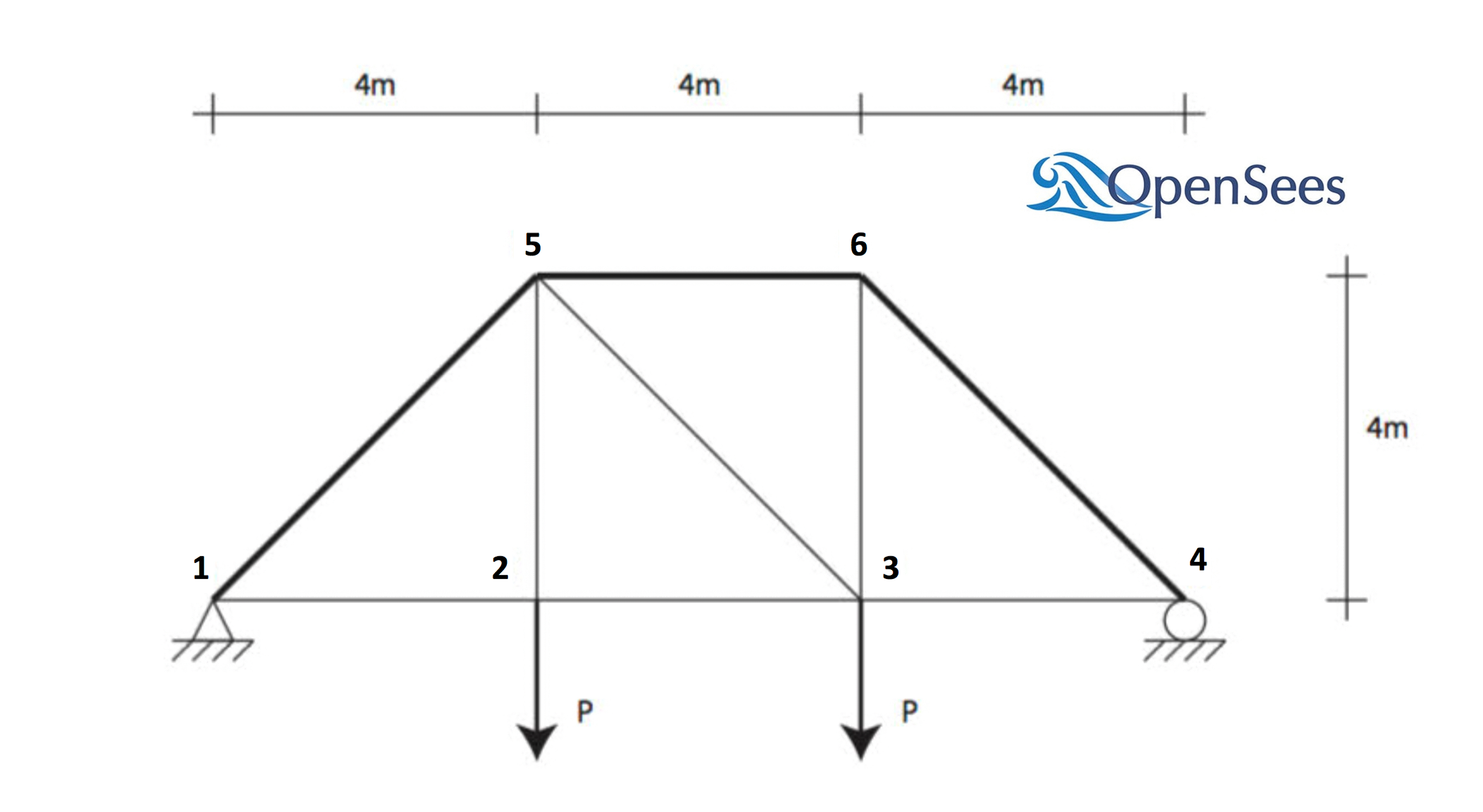
The structure has uncertain properties that all follow normal distribution:
Elastic modulus(
E): mean \(\mu_E=205 kN/{mm^2}\) and standard deviation \(\sigma_E =15 kN/{mm^2}\) (COV = 7.3%)Load (
P): mean \(\mu_P =25 kN\) and a standard deviation of \(\sigma_P = 3 kN\), (COV = 12%).Cross-sectional area for the upper three bars (
Au): mean \(\mu_{Au} = 500 mm^2\), and a standard deviation of \(\sigma_{Au} = 25mm^2\) (COV = 5%)Cross sectional area for the other six bars (
Ao): mean \(\mu_{Ao} = 250mm^2\), and \(\sigma_{Ao} = 10mm^2\) (COV = 4%)
The goal of the exercise is to estimate the mean and standard deviation of the vertical displacement at node 3.
The exercise requires two files. The user is required to download these files and place them in a **NEW* folder.* The two files are:
Main file: TrussTemplate.tcl
# units kN & mm

#
# set some parameters
#

pset E 205
pset P 25
pset Au 500
pset Ao 250

#
# build the model
#

model Basic -ndm 2 -ndf 2

node 1     0    0
node 2  4000    0
node 3  8000    0
node 4 12000    0
node 5  4000 4000
node 6  8000 4000

fix 1 1 1
fix 4 0 1

uniaxialMaterial Elastic 1 $E

element truss 1 1 2 $Ao 1
element truss 2 2 3 $Ao 1
element truss 3 3 4 $Ao 1
element truss 4 1 5 $Au 1
element truss 5 5 6 $Au 1
element truss 6 6 4 $Au 1
element truss 7 2 5 $Ao 1
element truss 8 3 6 $Ao 1
element truss 9 5 3 $Ao 1
timeSeries Linear 1
pattern Plain 1 1 {
    load 2 0 [expr -$P]
    load 3 0 [expr -$P]
}

#
# create a recorder
#

recorder Node -file node.out -scientific -precision 10 -node 1 2 3 4 5 6 -dof 1 2 disp

#
# build and perform the analysis
#

algorithm Linear
integrator LoadControl 1.0
system ProfileSPD
numberer RCM
constraints Plain
analysis Static
analyze 1

#
# remove the recorders
#

remove recorders
Note
The first lines containing pset will be read by the application when the file is selected and the application will autopopulate the Random Variables input panel with these same variable names. It is of course possible to explicitly use Random Variables without the pset command as is demonstrated in the verification section.
The TrussPost.tcl script shown below will accept as input any of the 6 nodes in the domain and for each of the two dof directions.
Postprocessing file: TrussPost.tcl.
# create file handler to write results to output & list into which we will put results
set resultFile [open results.out w]
set results []

# get list of valid nodeTags
set nodeTags [getNodeTags]

# for each quanity in list of QoI passed
#  - get nodeTag
#  - get nodal displacement if valid node, output 0.0 if not
#  - for valid node output displacement, note if dof not provided output 1'st dof

foreach edp $listQoI {
	set splitEDP [split $edp "_"]
	set nodeTag [lindex $splitEDP 1]
	if {$nodeTag in $nodeTags} {
	    set nodeDisp [nodeDisp $nodeTag]
	    if {[llength $splitEDP] == 3} {
		set result [expr abs([lindex $nodeDisp 0])]
	    } else {
		set result [expr abs([lindex $nodeDisp [expr [lindex $splitEDP 3]-1]])]
	    }
	} else {
	    set result 0.
	}
	lappend results $result
}

# send results to output file & close the file
puts $resultFile $results
close $resultFile
Note
The user has the option to provide no post-process script (in which case the main script must create a results.out file containing a single line with as many space separated numbers as QoI or the user may provide a Python script that also performs the postprocessing). Below is an example of a postprocessing Python script.
Alternative postprocessing file: TrussPost.py
#!/usr/bin/python

# written: fmk, adamzs 01/18

# import functions for Python 2.X support
from __future__ import division, print_function
import sys
if sys.version.startswith('2'):
    range=xrange
    string_types = basestring
else:
    string_types = str

import sys

def process_results(inputArgs):

    #
    # process output file "node.out" for nodal displacements
    #

    with open ('node.out', 'rt') as inFile:
        line = inFile.readline()
        displ = line.split()
        numNode = len(displ)

    inFile.close

    # now process the input args and write the results file

    outFile = open('results.out','w')

    # note for now assuming no ERROR in user data
    for i in inputArgs:

        theList=i.split('_')

        if (len(theList) == 4):
            dof = int(theList[3])
        else:
            dof = 1

        if (theList[0] == "Node"):
            nodeTag = int(theList[1])

            if (nodeTag > 0 and nodeTag <= numNode):
                if (theList[2] == "Disp"):
                    nodeDisp = abs(float(displ[((nodeTag-1)*2)+dof-1]))
                    outFile.write(str(nodeDisp))
                    outFile.write(' ')
                else:
                    outFile.write('0. ')
            else:
                outFile.write('0. ')
        else:
            outFile.write('0. ')

    outFile.close


if __name__ == "__main__":
    n = len(sys.argv)
    responses = []
    for i in range(1,n):
        responses.append(sys.argv[i])

    process_results(responses)
Warning
Do not place the files in your root, downloads, or desktop folder as when the application runs it will copy the contents on the directories and subdirectories containing these files multiple times. If you are like us, your root, Downloads or Documents folders contains an awful lot of files and when the backend workflow runs you will slowly find you will run out of disk space!
5.1.1. Sampling Analysis
Problem files |
To perform a sampling or forward propagation uncertainty analysis the user would perform the following steps:
Start the application and the UQ tab will be highlighted. In the panel for the UQ selection, keep the UQ engine as that selected, i.e. Dakota, and the UQ Method Category as Forward Propagation, and the Forward Propagation method as LHS (Latin Hypercube). Change the #samples to 1000 and the seed to 20 as shown in the figure.
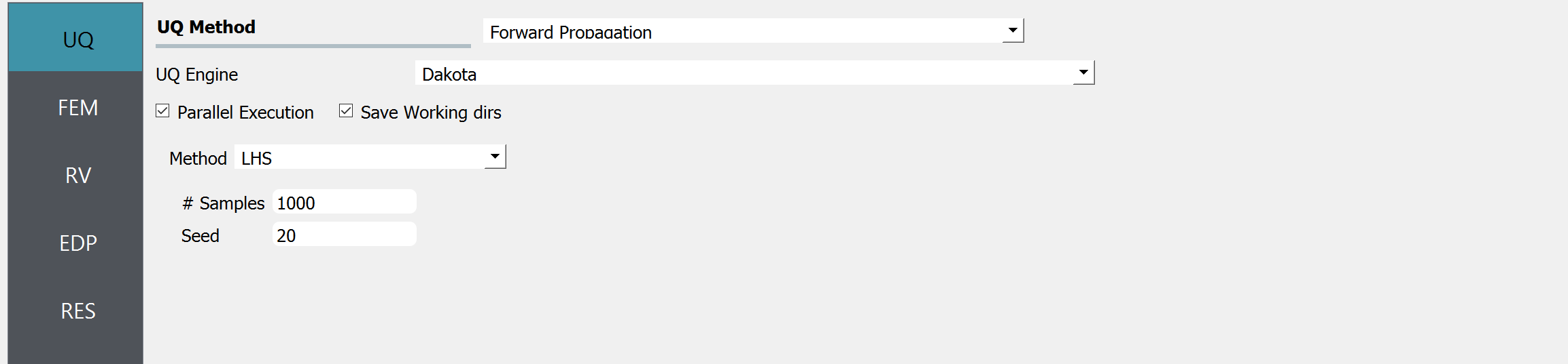
Sample size is related to the confidence interval of the estimates. Please refer to here.
Random seed is used to ensure that results are reproducible.
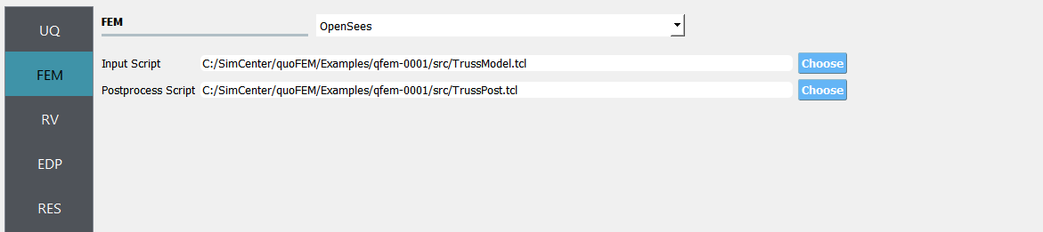
Next select the FEM panel from the input panel. This will default in the OpenSees FEM engine. For the main script copy the path name to
TrussModel.tclor select choose and navigate to the file. For the post-process script field, repeat the same procedure for theTrussPost.tclscript.
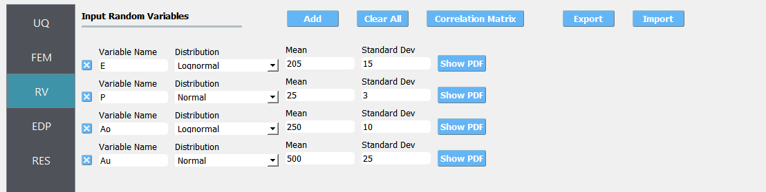
Next select the RV panel from the input panel. This should be pre-populated with four random variables with same names as those having
psetin the tcl script. For each variable, from the drop-down menu change them from having a constant distribution to a normal one and then provide the means and standard deviations specified for the problem.
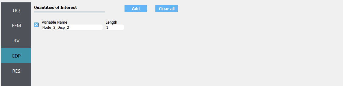
Next select the EDP panel. Here enter
Node_3_Disp_2for the one variable.
Note
The user can add additional QoI by selecting add and then providing additional names. As seen from the post-process script any of the 6 nodes may be specified and for any node either the 1 or 2 DOF direction.
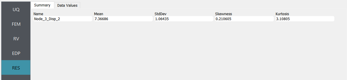
Next click on the Run button. This will cause the backend application to launch dakota. When done the RES panel will be selected and the results will be displayed. The results show the values the mean and standard deviation.
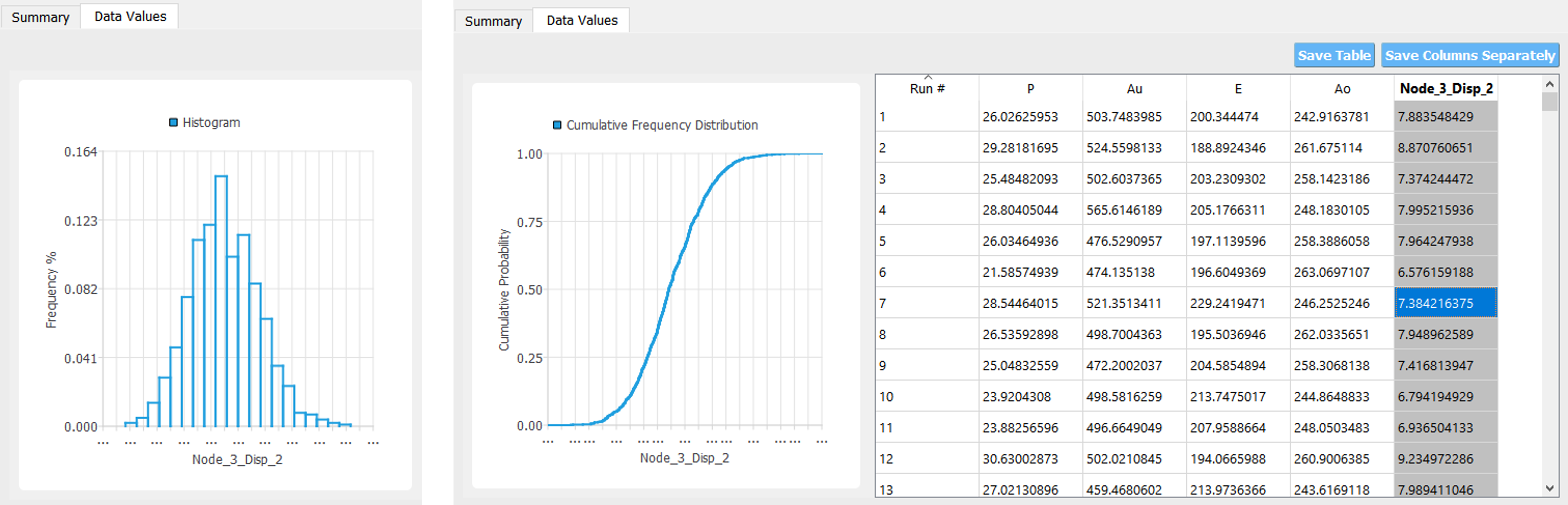
If the user selects the Data tab in the results panel, they will be presented with both a graphical plot and a tabular listing of the data.
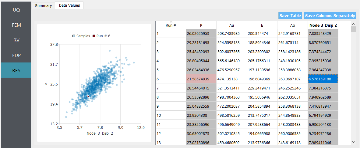
Various views of the graphical display can be obtained by left- and right-clicking in the columns of the tabular data. If a singular column of the tabular data is pressed with both right and left buttons a frequency and CDF will be displayed, as shown in figure below.
5.1.2. Reliability Analysis
Problem files |
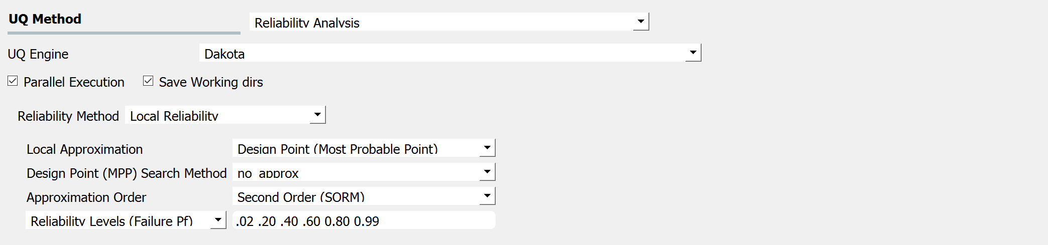
If one is interested in the probability that a particular response measure will be exceeded, an alternate strategy is to perform a reliability analysis. In order to perform a reliability analysis the steps above would be repeated with the exception that the user would select a reliability analysis method instead of a Forward Propagation method. To obtain reliability results using the Second-Order Reliability Method (SORM) for the truss problem the user would follow the same sequence of steps as previously. The difference would be in the UQ panel in which the user would select a Reliability as the Dakota Method Category and then choose Local reliability. In the figure the user is specifying that they are interested in the probability that the displacement will exceed certain response levels.
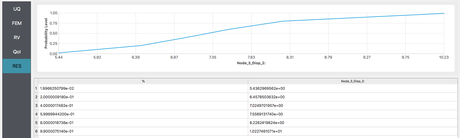
After the user fills in the rest of the tabs as per the previous section, the user would then press the RUN button. The application (after spinning for a while with the wheel of death) will present the user with the results.
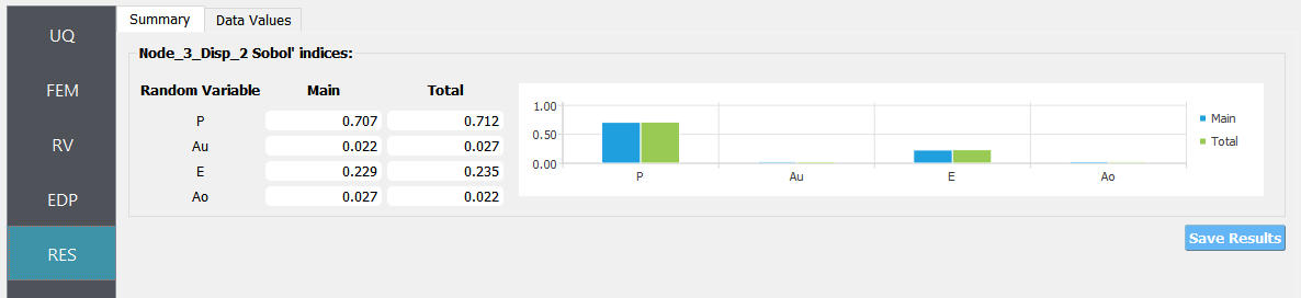
5.1.3. Global Sensitivity
Problem files |
In a global sensitivity analysis the user is wishing to understand what is the influence of the individual random variables on the quantities of interest. This is typically done before the user launches large scale forward uncertainty problems in order to limit the number of random variables used to limit the number of simulations performed.
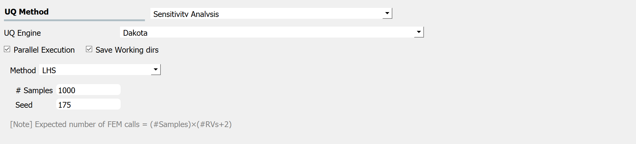
After the user fills in the rest of the tabs as per the previous section, the user would then press the RUN button. The application (after spinning for a while with the wheel of death) will present the user with the results.