5.3. Basic modeling with Python
Problem files |
This example illustrates how Python scripting can be used with quoFEM to express general mathematical models without the use of a dedicated finite element analysis engine.
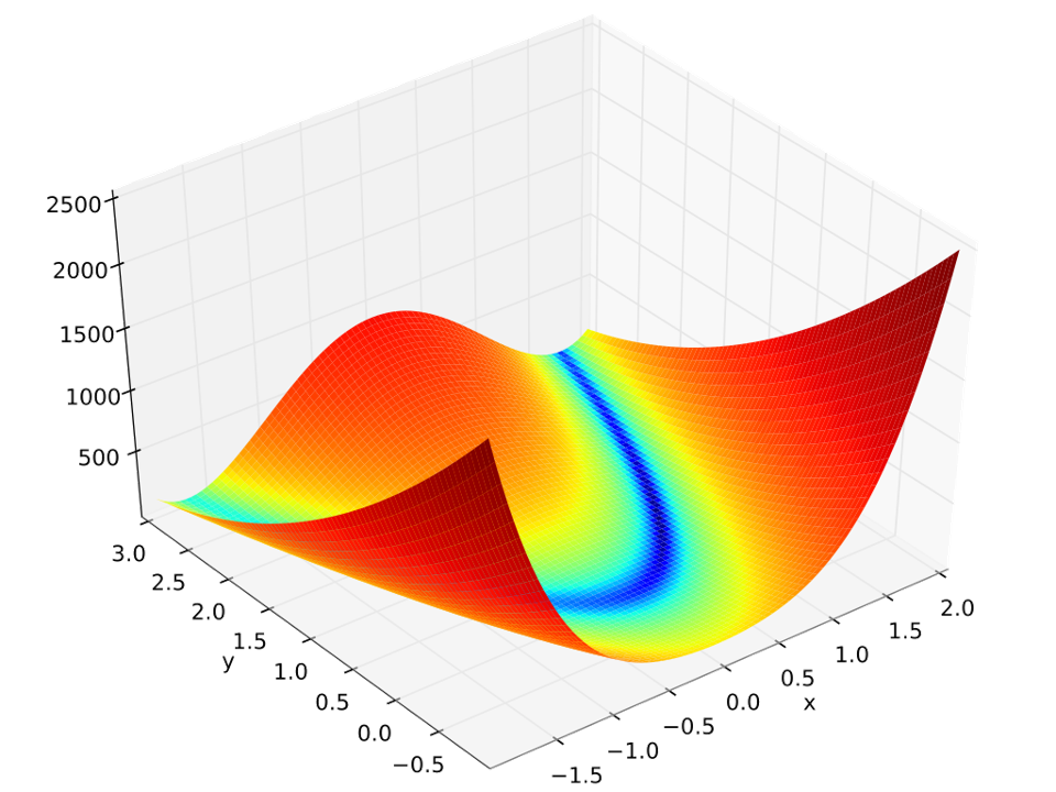
The Rosenbrock function is a test function that is often used to evaluate numerical optimization algorithms. It is given by the following expression:
A forward propagation analysis will be conducted to numerically integrate the first and second moments of a random variable whose value is obtained by applying the Rosenbrock function to the two following statistically independent random variables:
First variable,
X: Uniform distribution with a lower bound \((L_B)\) of \(-2.0\), upper bound \((U_B)\) of \(2.0\),Second variable,
Y: Uniform distribution with a lower bound \((L_B)\) of \(1.4\), upper bound \((U_B)\) of \(1.6\),
5.3.1. UQ Workflow
The objective of this UQ problem is to numerically integrate the following integrals with a forward propagation routine:
where \(f_{XY}(x,y)\) is the joint probability density function of the random variables \(X\) and \(Y\).
This procedure is implemented with a Latin hypercube sampling routine in quoFEM by entering the following inputs in the UQ tab:
Method |
LHS |
Samples |
200 |
Seed |
949 |
5.3.2. Model Files
For this forward propagation problem, we need to define a Python script
that will import a set of random variable values, apply them to the
Rosenbrock function, then write the results to a file named
results.out for every random variable realization generated by
Dakota. To this end, we begin by defining our random variables as Python
objects as follows, and supplying this as a .py script in the
Parameters File field of the FEM tab:
X = 0.0
Y = 0.0
Although this file will later be used as a Python module, it is important to note that in the quoFEM workflow, it is NOT handled as a true Python script. Rather, it can be thought of loosely as analogous to a C “header file” in that it simply gives us an interface to Dakota from Python. The values assigned to the variables at this point will not be used.
Note: The Parameters File is not a true Python script; For the time being, until further documentation about the tool is developed, users should only use line-by-line variable definitions in this file. Python assignments like
X, Y = 0.0, 0.0are not supported.
We can now implement our model for the Input File which will begin
with a star-import from the parameters file we just created. Assuming
that file was named params.py, this import would look like so:
from params import *
Next we define the following simple function which evaluates the Rosenbrock function:
def rosenbrock(x, y):
    a = 1.
    b = 100.
    return (a - x)**2.0 + b*(y - x**2.)**2.
Finally, we apply our rosenbrock function to the variables we
imported from params, and write the results to a file called
results.out. Note that throughout the forward propagation routine,
the values assigned to the variables X and Y in the params
interface are varied by the workflow application.
with open('results.out', 'w') as f:
    result = rosenbrock(X, Y)
    f.write('{:.60g}'.format(result))
The code from these steps is colleted and made available for download in the following files:
rosenbrock.py: This file is a Python script which implements the Rosenbrock function. It is supplied to the Input Script field of the FEM tab. Because this file writes directly to
results.out, it obviates the need for supplying a Postprocess Script. When invoked in the workflow, the Python routine is supplied a set of random variable realizations through the star-import of the script supplied to the Parameters File field.params.py: This file is a Python script which defines the problem’s random variables as objects in the Python runtime. It is supplied to the Parameters File field of the FEM tab. The literal values which are assigned to variables in this file will be varied at runtime by the UQ engine.