3.3. RV: Random Variables¶

The RV tab allows the user to specify the probabilistic distribution for the random problem at hand. The following probabilistic distributions for the random variables are currently supported:

3.3.1. Probability distribution¶

Note

To add a new random variable the user presses the Add button. To remove a random variable, the user must first select it by checking the small circle before the random variable, and then pressing the Remove button.

3.3.1.1. Dakota Engine¶

The following ten distribution classes are supported for the Dakota UQ engine.

Normal (Gaussian)

The user provides the mean ($\mu$) and standard deviation ($\sigma$) of the normal distribution. The density function of the normal distribution, as a function of $\mu$ and $\sigma$ is:

(3.3.1.1.1)¶\[f(x) = \frac{1}{\sqrt{2 \pi} \sigma} \exp \left( -{\frac{1}{2} \left( \frac{x - \mu}{\sigma} \right)^2} \right)\]
Lognormal

The user provides the mean ($\mu$) and standard deviation ($\sigma$) of the lognormal distribution. The density function of the lognormal distribution, as a function of $\mu$ and $\sigma$ is:

(3.3.1.1.2)¶\[f(x) = \frac{1}{\sqrt{2 \pi} \zeta x} \exp \left( -{\frac{1}{2} \left( \frac{\ln x - \lambda}{\zeta} \right)^2} \right)\]

where $\zeta^2 = \ln \left( \frac{\sigma^2}{\mu^2} + 1 \right)$ and $\lambda = \ln(\mu) - \frac{\zeta^2}{2}$
Beta

The user provides $\alpha$, $\beta$, lower bound ($L_B$), and an upper bound ($U_B$) for the beta distribution. The density function of the normal distribution, as a function of these quantities, is:

(3.3.1.1.3)¶\[f(x) = \frac{\Gamma(\alpha + \beta)}{\Gamma(\alpha)\Gamma(\beta)} \frac{(x - L_B)^{\alpha-1}(U_B-x)^{\beta-1}}{(U_B - L_B)^{\alpha + \beta - 1}}\]

where $\Gamma(\alpha)$ is the Gamma function.
Uniform

The user provides the lower bound ($L_B$), and an upper bound ($U_B$) for the uniform distribution. The density function of the normal distribution, as a function of these quantities, is:

(3.3.1.1.4)¶\[f(x) = \frac{1.0}{(U_B - L_B)}\]

The mean of the distribution is $\frac{(U_B + L_B)}{2.0}$
Weibull

The user provides the shape parameter ($k$) and scale parameter ($a_n$) for the Weibull distribution. The density function of the Weibull distribution, as a function of these quantities, is:

(3.3.1.1.5)¶\[f(x) = \frac{k}{a_n}\left(\frac{x}{a_n}\right)^{k-1} \exp \left( -(x/a_n)^{k} \right)\]

where $k,a_n > 0$ and $x \geq 0$. For $x<0$, $f(x) = 0$.
Gumbel

The user provides $\alpha$ and $\beta$ for the Gumbel distribution, where $\beta$ is known as the location parameter and $\frac{1}{\alpha}$ the scale parameter. The density function of the Gumbel distribution, as a function of these quantities, is:

(3.3.1.1.6)¶\[f(x) = \alpha e^{-\alpha(x-\beta)} \exp(-e^{-\alpha(x-\beta)})\]
Exponential

The user provides the parameter ($\lambda$) of the exponential distribution. The density function of the exponential distribution, as a function of $\lambda$, is:

(3.3.1.1.7)¶\[f(x) = \lambda \exp(-\lambda x)\]

where $x>0$ and $\lambda>0$. The user can alternatively provide the mean ($m$) of the exponential distribution.

(3.3.1.1.8)¶\[m = \frac{1}{\lambda}\]
Discrete

The user provides the $N$ discrete values ($x_i$) and their weights (probability $p_i$) for a multinomial distribution. The probability mass function of the discrete distribution is:

(3.3.1.1.9)¶\[\begin{split}p(x)=\begin{cases} p_i, & \text{if $x=x_i$}\\ 0, & \text{otherwise} \end{cases}\end{split}\]

where $p_i>0$. The weights ($p_i$) will be automatically normalized if they do not sum up to one. The option to define by moments is not supported for the discrete distribution.
Gamma

The user provides the shape parameter ($k$) and scale parameter ($\lambda$) of the Gamma distribution. The density function of the Gamma distribution, as a function of $k$ and $\lambda$, is:

(3.3.1.1.10)¶\[f(x) = \frac{\lambda^kx^{k-1}\exp(-\lambda x)}{\Gamma(k)}\]

where $\lambda>0$ and $k>0$. Users can alternatively provide the mean ($m$) and standard deviation ($\sigma$).

(3.3.1.1.11)¶\[\begin{split}m &= \frac{k}{\lambda} \\ \sigma &= \sqrt{\frac{k}{\lambda^2}}\end{split}\]
Chi-squared

The user provides the parameter $k$ of the Chi-squared distribution. The density function of the Chi-squared distribution, as a function of $k$, is

(3.3.1.1.12)¶\[f(x) = \frac{1}{2^{\frac{k}{2}}\Gamma\left(\frac{k}{2}\right)}x^{\left(\frac{k}{2}-1\right)} \exp\left(-\frac{x}{2}\right)\]

where $x>0$ and $k$ is a natural number. Users can alternatively select the moment option where the mean ($m$) is

(3.3.1.1.13)¶\[m = k\]

For each random variable, the user must enter a name and select from the drop-down menu the distribution associated with the random variable. For the distribution selected, the user must then provide the input arguments, which are as described above. Fig. 3.3.1.1.1 shows the panel for a problem with four Random Variables with all random input following Gaussian distributions.

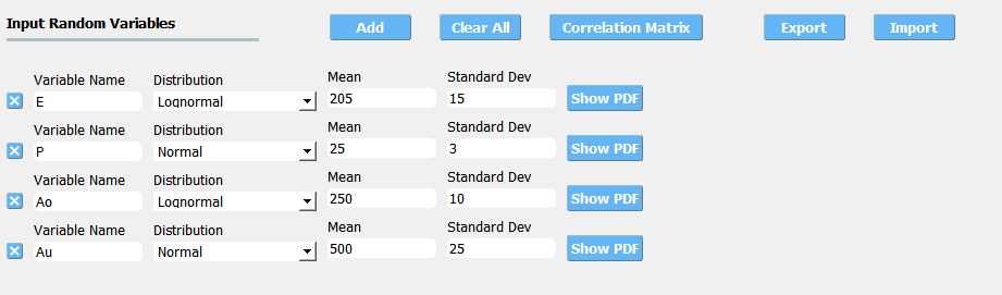
Fig. 3.3.1.1.1 Random variable specification.¶

Note

To add a new random variable the user presses the Add button. To remove a random variable, the user must first select it by checking the small circle before the random variable, and then pressing the Remove button.

Warning

Removing a random variable may have unintended consequences and cause the UQ engine to fail.

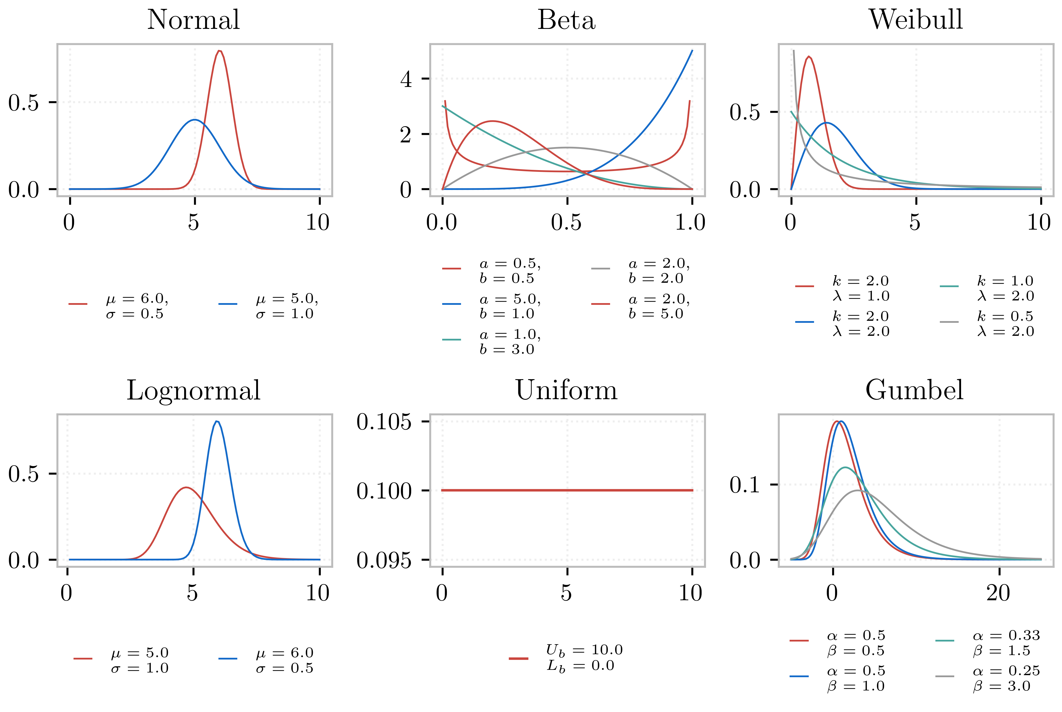
Fig. 3.3.1.1.2 Distributions offered by the quoFEM app.¶

3.3.1.2. SimCenterUQ Engine¶

One additional distribution is supported in the SimCenter UQ engine. The users can also define distributions either by Parameters, Moments or Dataset. (Note: Nataf transform module developed by [ERA19] is adopted)

Truncated exponential

The user provides the parameter $k$ and bounds $L_B$ and $U_B$ for the truncated exponential distribution. The density function of the truncated exponential distribution is

(3.3.1.2.1)¶\[f(x) = \frac{\lambda}{c} \exp(-\lambda x), \text{ where $L_B<x<U_B$}\]

where $c$ is a normalization constant, i.e.

(3.3.1.2.2)¶\[c = \int_{L_B}^{U_B} \lambda\exp(-\lambda x) dx\]

where $x>0$ and $\lambda>0$. Users can alternatively provide the mean of the distribution along with the truncated bounds.

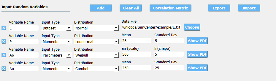
Fig. 3.3.1.2.1 Extended random variable specification¶

Input Type - Dataset

Users can also define the random variables by providing a sample realization data set as shown in the below figure, by selecting the Dataset input type. The data will be fitted to the specified probability distribution model. Note that for some bounded distributions, such as beta and truncated exponential, the bounds should additionally be provided through the user interface.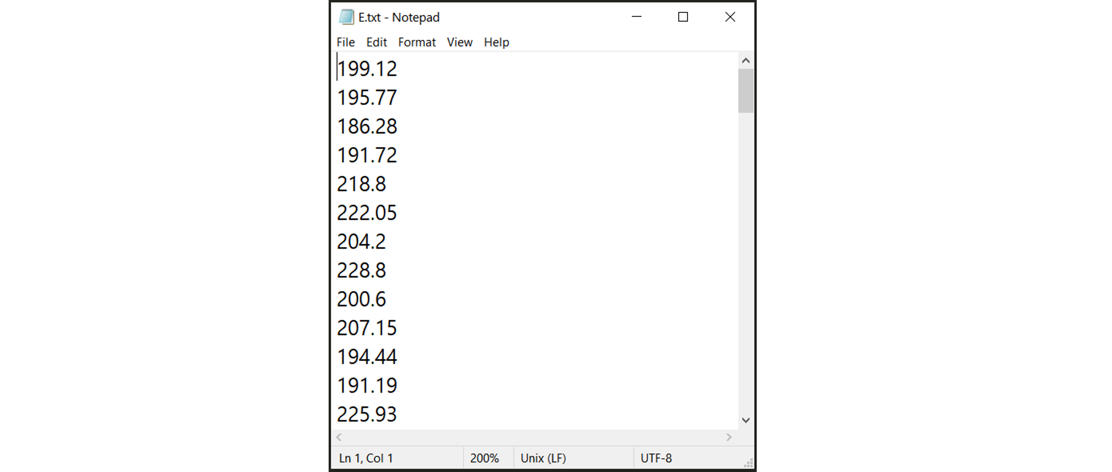

Fig. 3.3.1.2.2 Example of the input dataset file¶
Note
- Clicking the Show PDF or Show PMF button will display the probability distribution (or mass) function of each random variable with the specified parameters/moments. If the PDF or PMF is not displayed, we recommend the users double-check if the parameters/moments are in a valid range. The plotting button is not activated for the Dataset input type.
ERA19

Engineering Risk Analysis Group, Technische Universität München: https://www.bgu.tum.de/era/software/eradist/ (Matlab/python programs and documentations)

Correlation coefficients between each variable can be defined by clicking the Correlation Matrix button. Default correlations between variables are set to zero. The diagonal element of the matrix is fixed as one, and symmetry of the correlation matrix is enforced once the entries of the lower triangular part of the matrix are modified.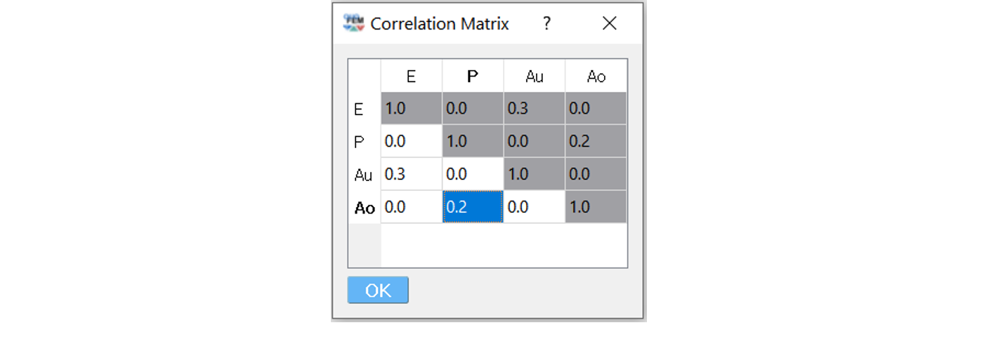

Fig. 3.3.1.2.3 Example of a valid correlation matrix¶

Once the OK button is clicked after setting all required entries, the program will automatically check the validity of the matrix before closing the correlation matrix window. If the matrix is not positive definite, an error message will be displayed and the window will not be closed. In such a case, the user should adjust the correlation coefficients to be positive definite.
Note
- When a constant variable is introduced instead of probability distributions, the correlation coefficient corresponding to those variables will be ignored.
- When more than one random variable is provided as Dataset, correlations between the data pairs will not be incorporated automatically. If correlations exist, the user can define them manually at the correlation matrix window.
Warning

Correlation warping for Nataf variable transformation of beta distributions is currently not supported.

Tip

Summary of capabilities and limitations

o Specify 12 different kinds of random distributions either by parameters, moments (mean and variance), or data samples (Specify 7 different kinds of random distributions by parameters when using Dakota instead of SimCenterUQ)
o Draw correlated samples through Nataf transformation (Gaussian-copular)
x Explicitly specify random fields (planned)
x Specify user-defined random distribution (planned)
x Specify Non-Gaussian copular correlation (upon request)

3.3.1.3. UCSD-UQ Engine¶

The same set of distributions that are supported by the SimCenterUQ engine are supported in the UCSD-UQ engine. Currently, the distributions can only be defined through their Parameters. Correlation between the random variables is not supported in the UCSD-UQ engine.

3.3.1.4. CustomUQ Engine¶

The same set of distributions and correlation options as that supported by the SimCenterUQ engine can also be selected when the CustomUQ engine is used. Additionally, two options - User defined and User defined vector are also available.

When the User defined option is chosen, the user must provide the path to a script file that makes the desired functionality for the CustomUQ engine available, such as methods to draw samples from the user-defined distribution, or to evaluate the probability density of the user-defined distribution at specified sample points, etc.

When the User defined vector option is chosen, in addition to the path to the script file, the user must also enter the number of components in the random vector.

../../../../_images/userDefinedDists.png

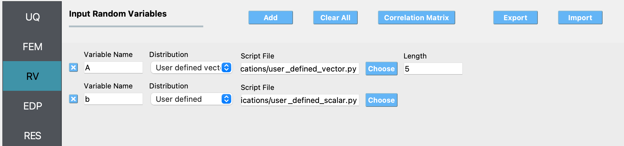
Fig. 3.3.1.4.1 Specifying user-defined distributions under the CustomUQ engine¶

3.3.2. Video Resources¶

Recorded in tool training, 2022.