3.9. Verification Results

This page summarizes sample results from the testbed runs with an emphasis on verifying the estimated loss ratios by hand calculations.

3.9.1. Building Inventory

From the entire building inventory, 98 buildings are randomly selected (examples are shown in Table 3.9.1.1 and the full inventory can be accessed here). Fig. 3.9.1.1 shows the data distributions of the built year, surface roughness (i.e., Terrain), roof shape, number of stories, and occupancy class.

Table 3.9.1.1 Example sampled building inventory

ID	RoofShape	FloodZone	Area	Longitude	Latitude	Terrain	DWSII	BuildingType	OccupancyClass	AvgJanTemp	Garage	RoofSlope	NumberofStories	MeanRoofHt	YearBuilt
1	Gable	X	478	-93.24	30.14	76	133.1	Wood	RES1	Above	1	0.03	1	12.6	1991
2	Gable	X	358	-93.24	30.14	24	133.1	Wood	RES1	Above	1	0.07	1	13.3	1992
3	Gable	X	292	-93.24	30.13	76	133.3	Wood	RES1	Above	1	0.31	2	29.6	1987
4	Gable	X	151	-93.24	30.14	76	133.2	Wood	RES1	Above	0	0.11	1	14	1990
5	Gable	X	519	-93.24	30.13	76	133.2	Wood	RES1	Above	0	0.07	1	13.2	1988
6	Hip	X	559	-93.24	30.14	76	133.1	Wood	RES1	Above	0	0.1	1	13.7	1989
7	Hip	X	427	-93.24	30.14	76	133.2	Wood	RES1	Above	1	0.22	1	15.9	1988
8	Hip	X	607	-93.24	30.14	76	133.1	Wood	RES1	Above	1	0.26	1	16.7	1990
9	Hip	X	544	-93.24	30.14	24	133.1	Wood	RES1	Above	0	0.16	1	14.9	1989
10	Gable	X	469	-93.24	30.13	76	133.2	Wood	RES1	Above	1	0.06	1	13	1990
11	Hip	X	458	-93.24	30.14	76	133.2	Wood	RES1	Above	0	0.14	1	14.6	1988
12	Hip	X	742	-93.24	30.14	24	133.1	Wood	RES1	Above	0	0.25	1	16.5	1992
13	Gable	X	524	-93.24	30.13	76	133.2	Wood	RES1	Above	0	0.17	2	27	1988
14	Gable	X	442	-93.24	30.14	76	133.1	Wood	RES1	Above	0	0.24	1	16.4	1991
15	Flat	X	515	-93.24	30.14	76	133.1	Wood	RES1	Above	0	0	1	12	1992
16	Gable	X	453	-93.24	30.13	76	133.3	Wood	RES1	Above	0	0.19	2	27.4	1989
17	Gable	X	455	-93.24	30.13	21	133.2	Wood	RES1	Above	0	0.06	1	13.1	1988
18	Hip	X	378	-93.24	30.14	76	133.1	Wood	RES1	Above	1	0.14	1	14.6	1987
19	Gable	X	507	-93.24	30.13	21	133.2	Wood	RES1	Above	0	0.32	1	17.8	1988
20	Gable	X	605	-93.24	30.14	21	133.1	Wood	RES1	Above	0	0.28	1	17	1987

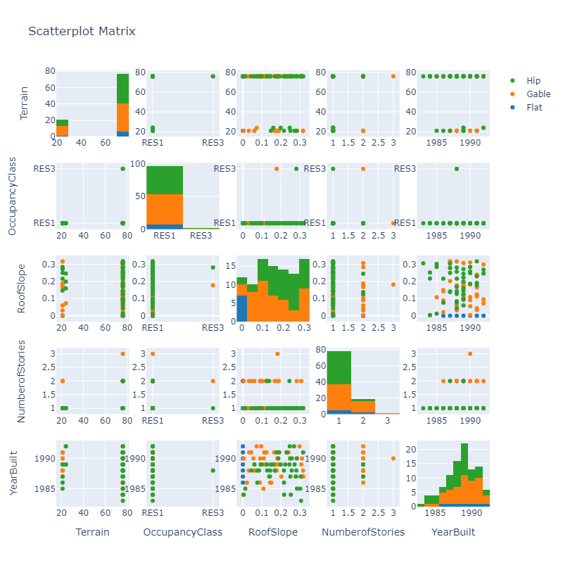
Fig. 3.9.1.1 Scatter matrix of sampled buildings.

3.9.2. Hand Calculation

Hand calculations of wind loss ratios are conducted using the input building information and intensity measures for the sampled buildings. Note that there are two major processes in the damage and loss assessment: (1) translating the building inventory to corresponding HAZUS building classes and (2) estimating the damage and loss given the HAZUS building class and the intensity measure (i.e., PWS in this testbed) for each building. The first process will be discussed in Verification of Rulesets. The second process is addressed by this section with key steps:

1. Mapping the building inventory to HAZUS building classes using the AssetRepresentationRulesets

2. Fetching the individual damage fragilities and loss ratios for each building given its HAZUS building class

3. Sampling the PWS from nearby grid sites

4. Evaluating the damage states and average loss ratio given the damage and loss functions as well as the sampled PWS

Following these steps, Fig. 3.9.2.1 compares the hand-calculated loss ratios and the simulated results, which are in good agreement.

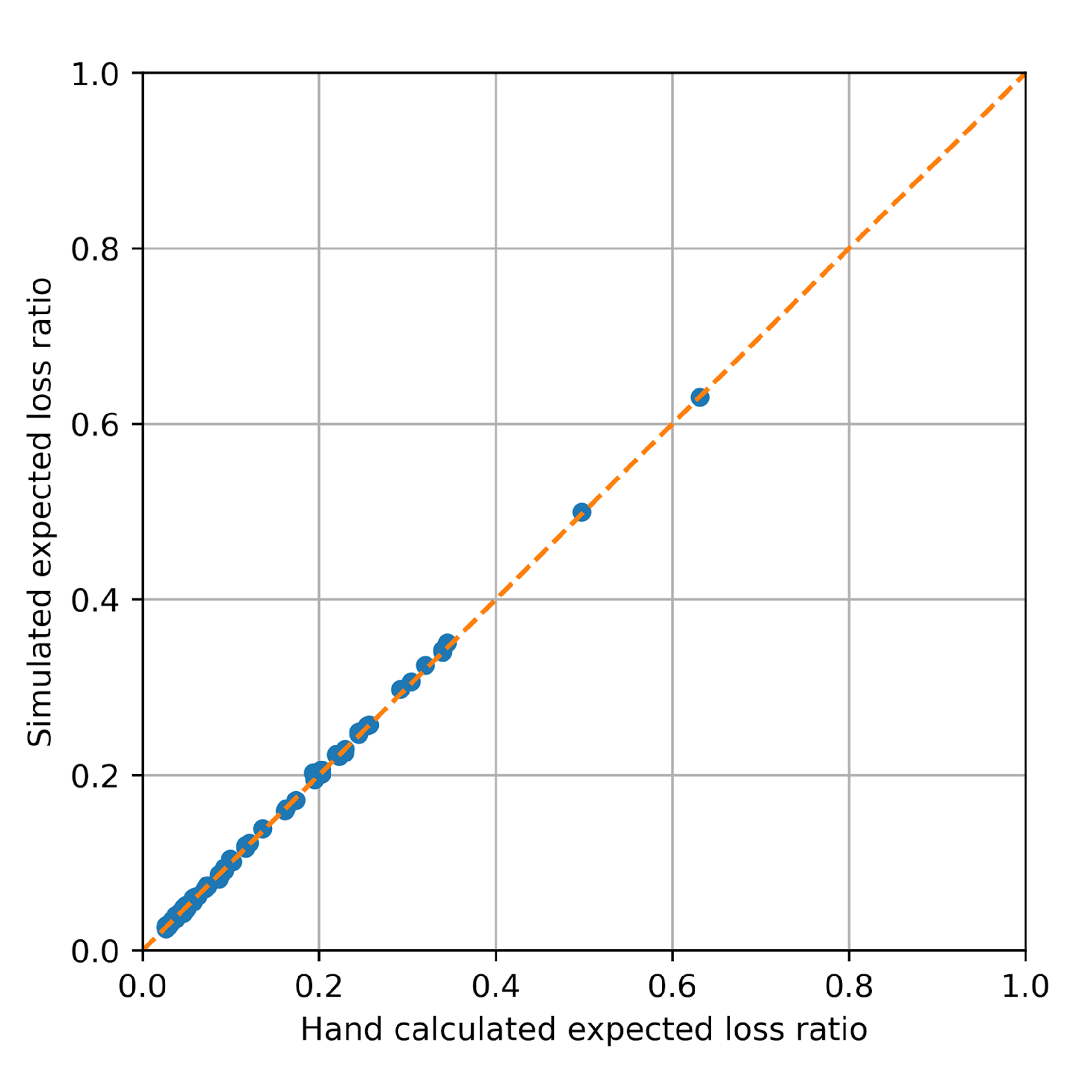
Fig. 3.9.2.1 Hand-calculated results vs. simulated results.

3.9.3. Verification of Rulesets

Following the discussion in the previous section, this section discusses the verification process for the rulesets introduced in Asset Representation. This verification includes two aspects: (1) verifying the implementation of rulesets and (2) verifying the influence of rulesets. The first aspect is addressed by the pytest module in the AssetRepresentationRulesets. Each pytest examines a set of rulesets for a specific HAZUS building class to see if the resulting HAZUS classifier is as expected. The second aspect involves examinations of damage and loss results from the testbed to investigate the influence of a specific building attribute on the building performance, i.e., if the results are rational then the corresponding rulesets are verified. As an example of this process, the construction year (YearBuilt) is focused in this section.

In order to investigate the cause and rationalize potential influence of year built, a parametric study is conducted for a single-family house (ID = 2 in Table 3.2.4.1). The original building record is expanded to 51 different buildings by varying the year built only (i.e., from 1970 to 2020). For each building, the expected loss ratio is estimated with 50 realizations to consider the uncertainty from the random sampling in the rulesets. The black curves in Fig. 3.9.3.1 plot the individual realizations of expected loss ratio against different year built values. The red curve shows the mean value based on the 50 realizations at each year built. It is clear to see that the building performance improves following major code revisions. For example, labeled by the yellow dashed line at 2000, the IRC 2000-2009 requires 8d nails (with spacing 6”/6”) for sheathing thickness of 1” (as default in this testbed) for basic wind speeds greater than 100 mph which enhances the building performance (reducing the loss ratio); while this ultimate wind speed is increased to 130 mph (just above the DWSII of the building) after 2016 accepting the use of spacing to 6”/12” which in turn slightly degrades the building performance. This observation highlights the particular importance of nail spacing requirements for sheathing in reducing wind-induced losses for this class of building.

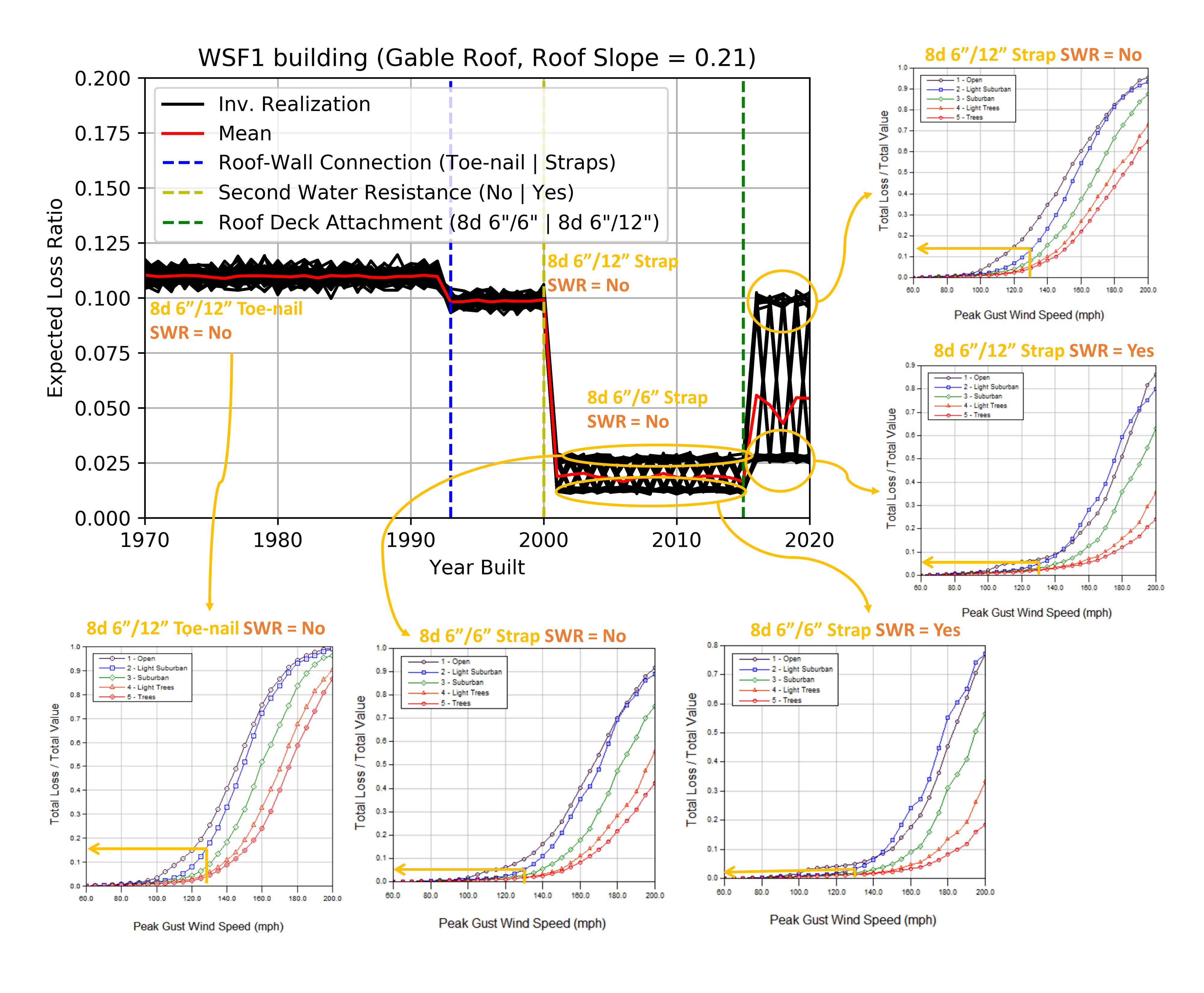
Fig. 3.9.3.1 Expected loss ratio vs. year built (WSF1, Gable Roof, Roof Slope=0.21)

A similar study is also conducted for a multi-unit wood building (i.e., WMUH1) with the year of construction varying from 1970 to 2020. For each building, the expected loss ratio is estimated with 50 realizations to consider the uncertainty from the random sampling in the rulesets. Fig. 3.9.3.2 plots individual realizations of expected loss ratio in black and the average in red. Two year divisions (1987 and 2000) are noticeable where buildings are estimated to have different performances. Further investigation into the cause of this trend indicates that the buildings from 1988 to 2000 are classified by our ruleset to have the second water resistance (SWR) given the roof slope is less than 0.33, whereas for the pre-1988 and post-2000 buildings, random samplings are conducted to assign SWR to the building by chance (30% for pre-1988 and 60% for post-2000, which also explains that on average the expected loss after 2000 is lower than the expected loss before 1988).

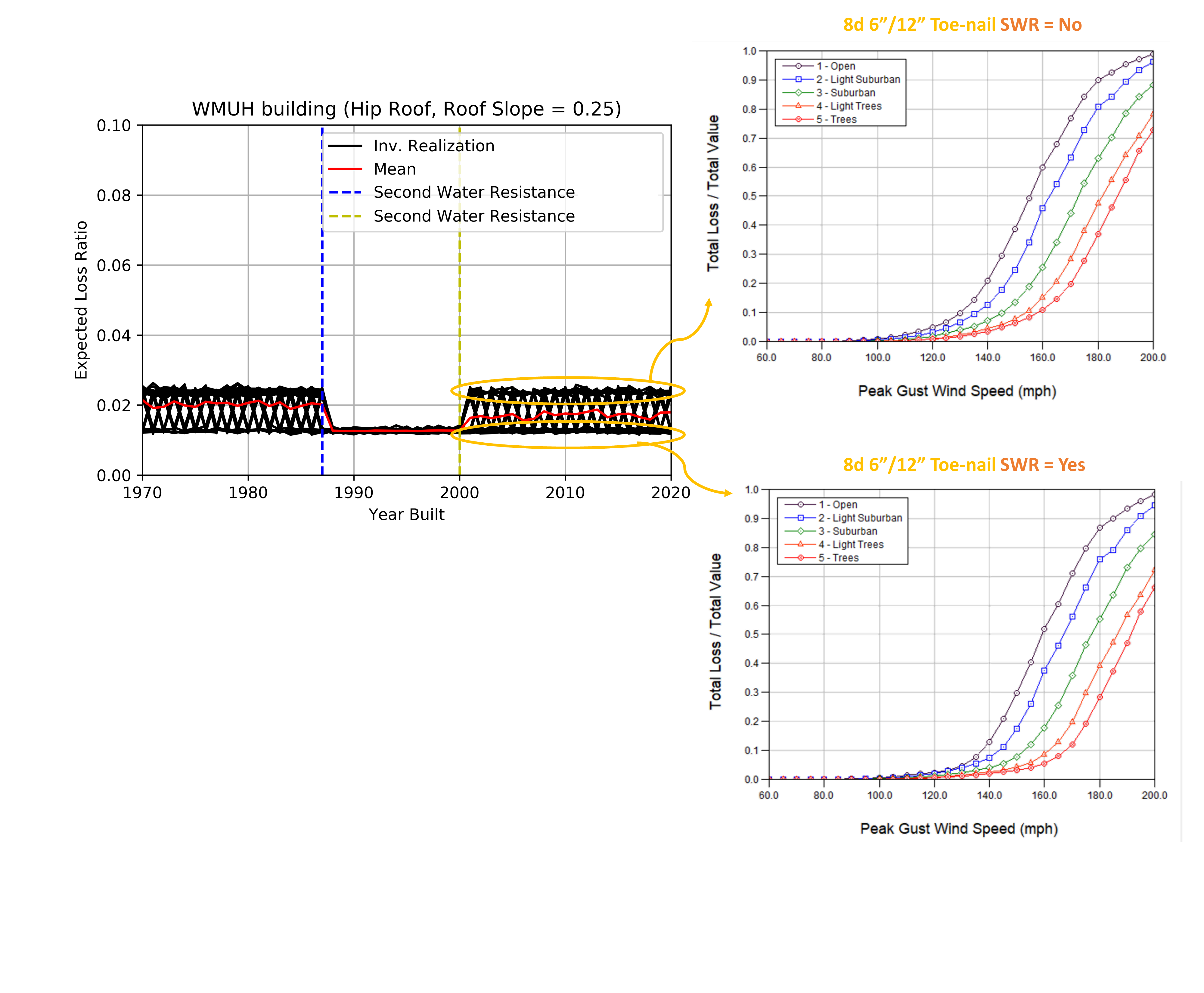
Fig. 3.9.3.2 Expected loss ratio vs. year built (WMUH1, Hip Roof, Roof Slope=0.25)