3.1.3.1. Forward Propagation
The forward propagation provides a probabilistic understanding of output variables by producing sample realizations and statistical moments (mean, standard deviation, skewness, and kurtosis). Currently, only the Monte Carlo Sampling (MCS) method is available in the SimCenterUQ engine and the other sampling methods (Latin hypercube sampling, Surrogate model-based efficient sampling) are available in the Dakota engine.
Sampling from dataset
SimCenterUQ uniquely provides an option to define the distribution of random variables (RVs) directly from the samples of the RVs (See RV: Random Variables). This feature is useful when the user does not know the actual distribution of an RV but has sample realizations. When a dataset is provided, quoFEM either treats the data as a discrete distribution (when Discrete distribution option is selected) or fits a parametric distribution to the data (when another distribution option is selected). For the former case, quoFEM uniformly samples the discrete index of the dataset provided by the user and uses the value corresponding to the index for the forward propagation analysis. The index is sampled either with replacement if the data size is smaller than the number of samples to draw or without replacement if the data size is larger than the number of samples to draw. Further, when the user provides coupled samples of correlated RVs, vector-wise resampling can be performed instead of independent resampling. In particular, a single index is sampled and shared in multiple variables for each realization.
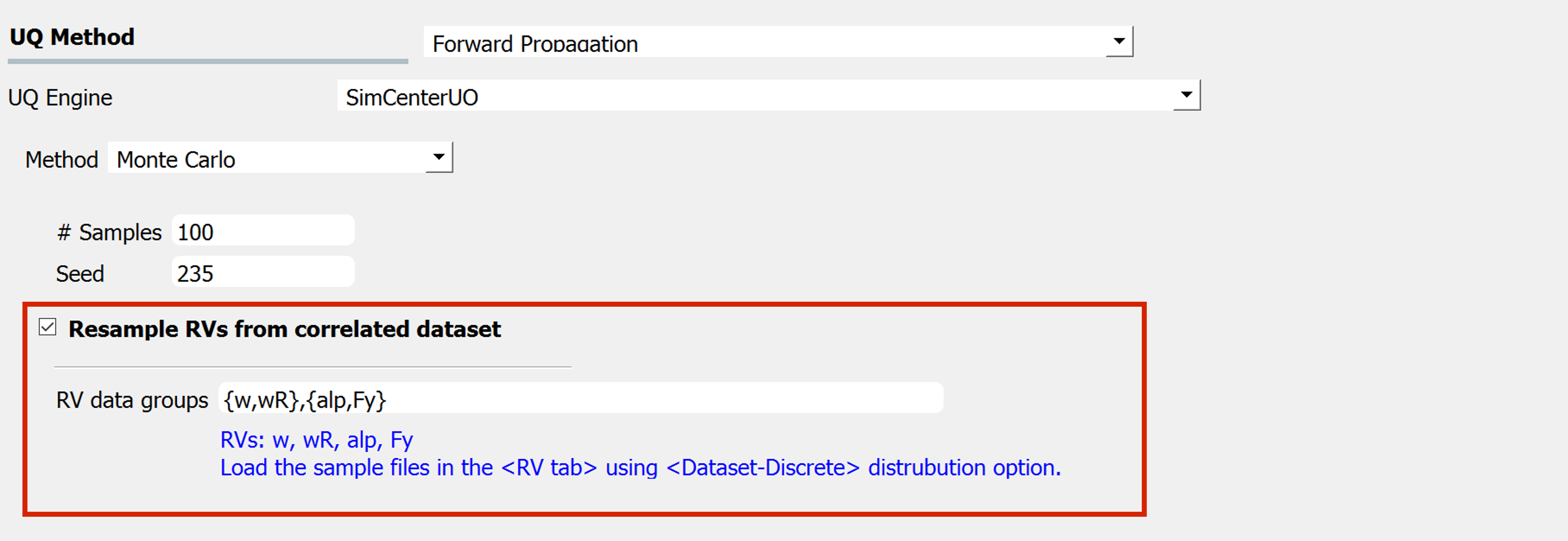
Click the checkbox to import correlated datasets
To enable this feature, the user can explicitly define the group of RVs that will share the index samples in the UQ tab using the Resample RVs from correlated dataset:
The actual datasets of the RVs written in this field should be imported in the RV tab, through the
parameters-discreteoption.The RVs inside each group should be provided with the same length of the samples (e.g. in
figSimSamp3, \(w\) and \(wR\) should have the same sample size \(N_1\) and \(alp\) and \(F_y\) should have the same sample size \(N_2\))
Note
Any correlation values for this coupled datasets additionally specified in the RV tab will be ignored. Note that the correlation of the data is already reflected in the analysis by introducing the same resampling index.
For example, consider the case where two variables \(w\) and \(wR\) are provided as 10 discrete data points in the RV tab as in Fig. 3.1.3.1.1.
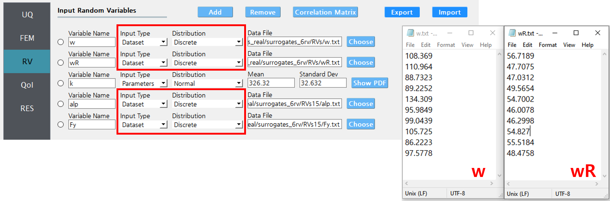
Fig. 3.1.3.1.1 Example RV tab. The RVs \(w\) and \(wR\) have the same sample size when they are specified to be coupled as shown in figSimSamp3.
Below is an example of 100 realizations of the two variables when they are considered to be independent, i.e. without checking the “Resample RVs from correlated dataset” option.
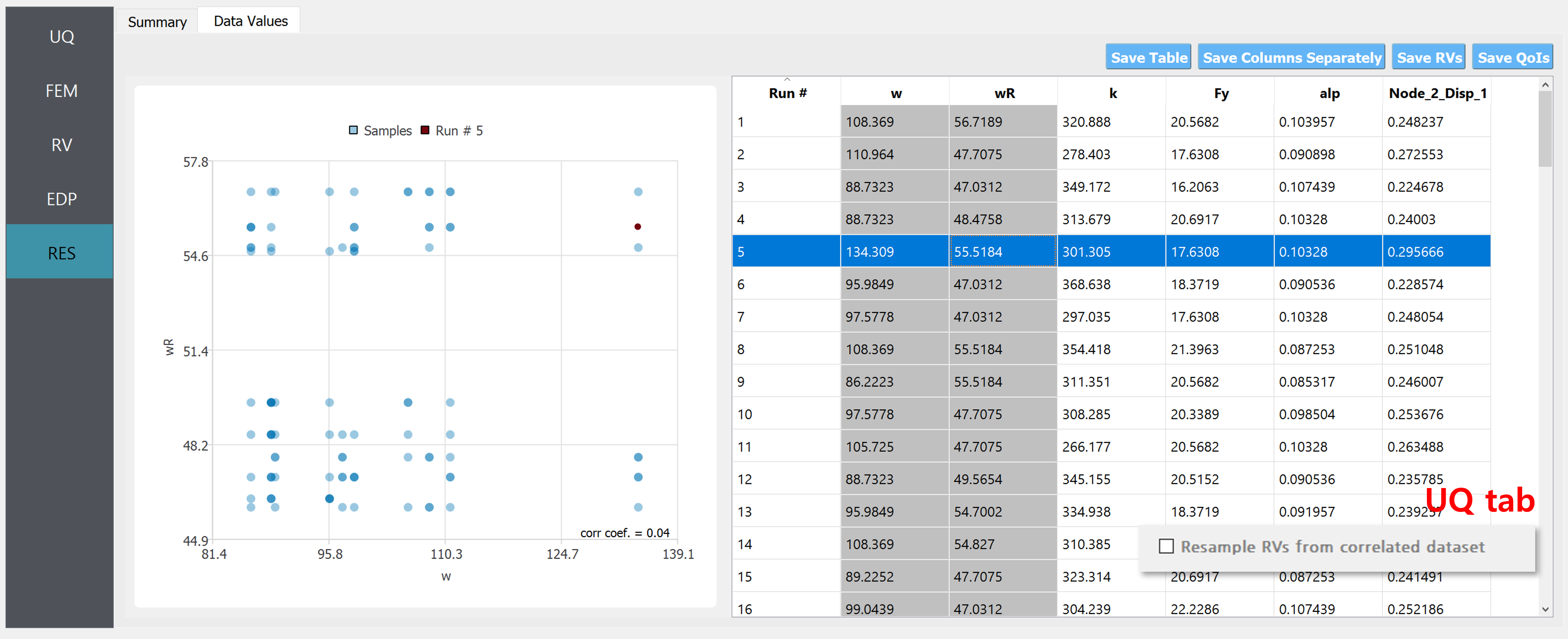
Fig. 3.1.3.1.2 Example of correlated samples (when the “Resample …” option in the UQ tab is enabled).
On the other hand, if the two datasets are considered correlated, i.e. if “Resample RVs from correlated dataset” are checked and the group {w,wR} is reported in the field as shown in figSimSamp3, 100 realization pairs of the RVs will be stacked on top of the provided 10 data points.
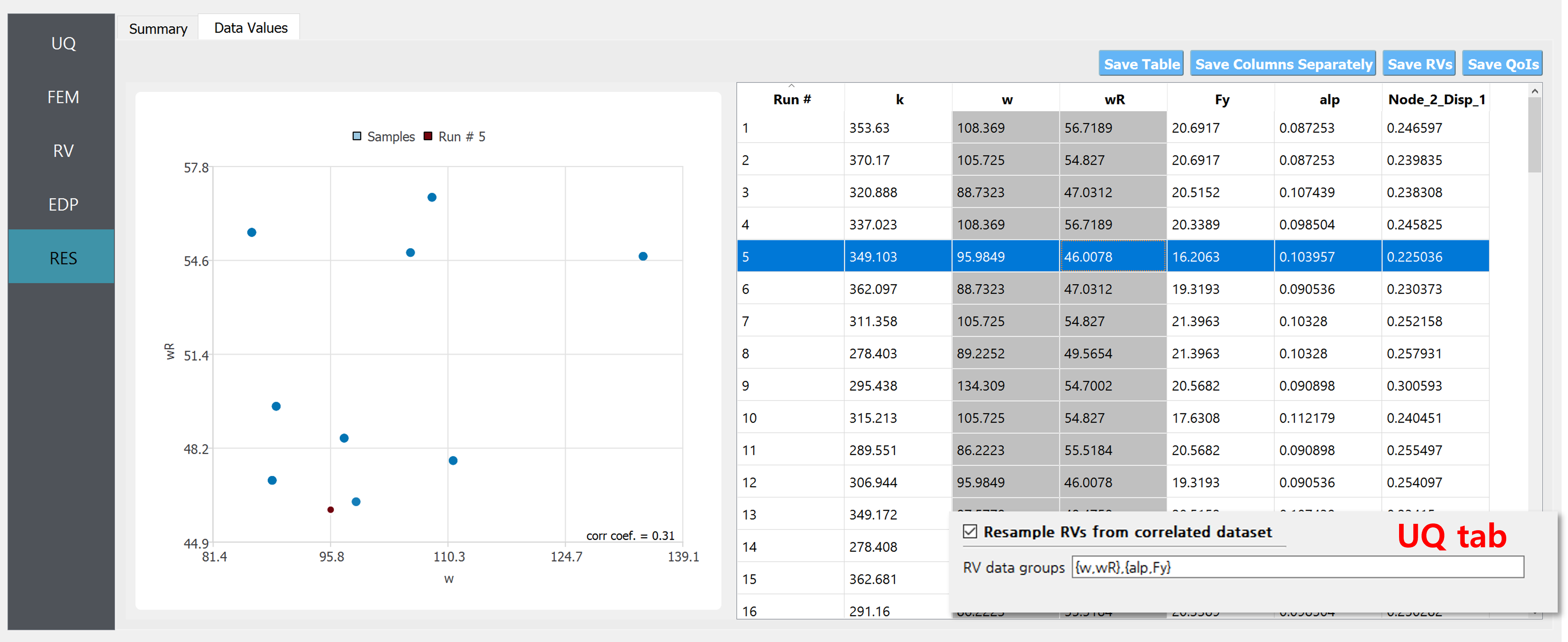
Fig. 3.1.3.1.3 Example of uncorrelated samples (when the “Resample …” option in the UQ tab is enabled).
This feature is especially useful when the user wants to perform a forward UQ analysis directly using the posterior samples obtained from Markov Chain Monte Carlo or other Bayesian sampling approaches.
Tip
Summary of capabilities and limitations
o Run Monte Carlo simulation for 12 different kinds of probability distributions with correlations.
o Use data samples as discrete distribution (especially useful when propagating samples from Bayesian updating)
x Run advanced sampling algorithms including Latin hypercube and surrogate-aided sampling. [Available in Dakota engine]
Multi-fidelity Monte Carlo
SimCenter UQ supports a multi-fidelity Monte Carlo option, where the user can import both high-fidelity and low-fidelity simulation models to estimate the statistics of high-fidelity models. See more information in the technical manual.
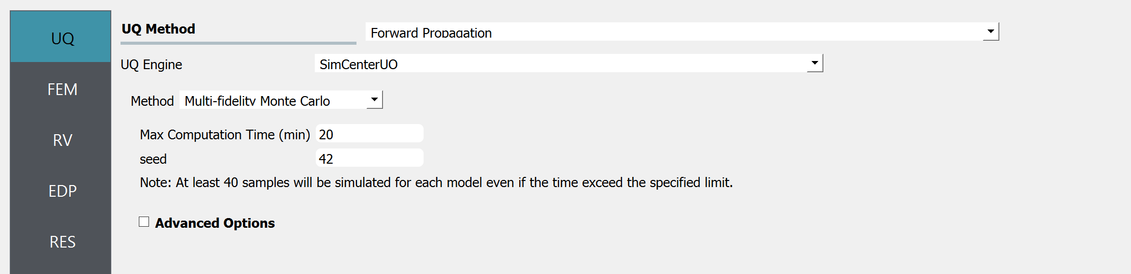
Fig. 3.1.3.1.4 Multi-fidelity Monte Carlo
The users should define Max Computation time and Seed
Max Computation Time (minutes): The target computation time for the analysis. Note that this is a “soft” target, meaning the analysis may not necessarily be completed within the specified time limit. The total number of simulations is decided after a few pilot runs of simulations considering the remaining budgets (time), and the process is not enforced to finish even if the target time is exceeded. Therefore, there could be a few minutes of estimation error in the max computation time. Note that, even if the specific time is exceeded, the analysis will not end until the minimum number of specified simulations (default is 40) is reached.
Seed: a positive integer that is used to reproduce the exact sequence of the pseudo-random number generator. The seed is to ensure the reproducibility of the results.
Additionally, advanced options can be selected by checking the option at the bottom

Fig. 3.1.3.1.5 Advanced options
Using the advanced options, the user can define the minimum number of simulations per model and an option to Perform log-transform
Minimum # simulations per model: The number of pilot samples. The pilot samples are used to estimate the correlations between the high- and low-fidelity models and decide the optimal number of simulations given the time limit. See here for more details. By default, the minimum number of simulations is 40.
Perform log-transform: Estimate the mean and variance of the log-transformed value (natural logarithm or \(ln()\) instead of \(log_{10}()\)). In quoFEM, the default is unchecked.