3.7. Target Spectrum by Surrogate Hazard GP Model

In some cases, users may want to specify the target response spectrum in ground motion selection using a pre-trained surrogate hazard model. This example demonstrates using quoFEM-trained Gaussian Process hazard model to get a target response spectrum at a specific site location in the San Francisco Bay Area given the seismicity from the Hayward Fault.

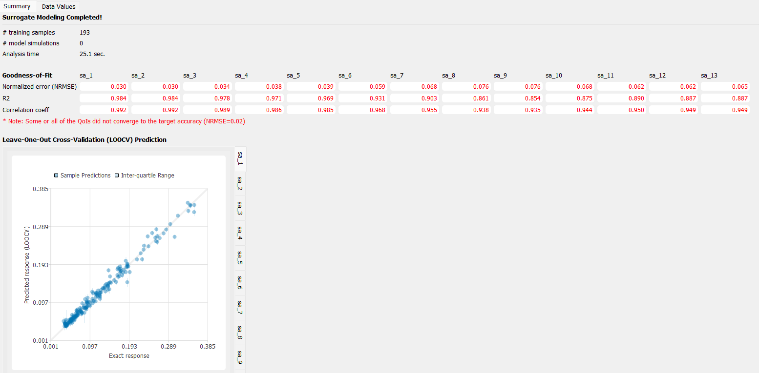
3.7.1. Pre-trained Gaussian Process Surrogate Model

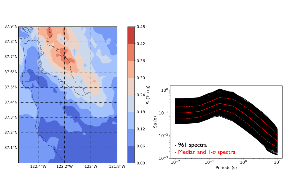
1. In this example, the Gaussian Process (GP) model is trained on regional earthquake intensity measure maps that are generated for 147 possible Hayward earthquake scenarios in the UCERF-2 model. For each scenario, the response spectral accelerations at periods from 0.01 sec to 10.0 sec are evaluated for overall 961 sites (31 times 31) in the San Francisco Bay Area. Inter-event and intra-event correlations are considered for all the sites whose median spectra are used as the training dataset.

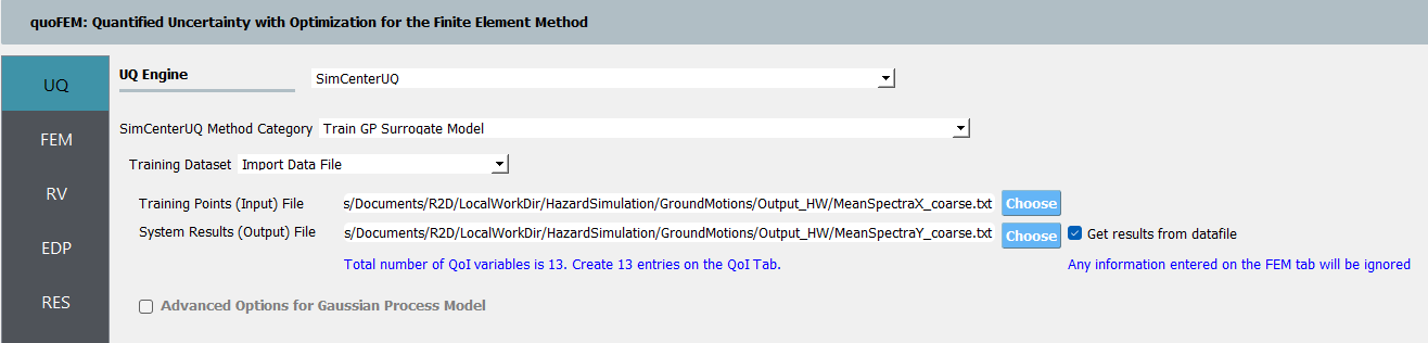
2. The training dataset (X.txt and Y.txt) is then loaded in quoFEM to train a GP model where the Longitude and Latitude are input variables and the median response spectrum at that site location is the output. The training takes about 25 sec and shows good performance and accuracy in the cross-validation. The trained model is saved into two files (SimGpModel.json and SimGpModel.pkl) for the use in EE-UQ.

3.7.2. Configure Surrogate Target Spectrum

1. Navigate to the EVT tab and select the PEER NGA Records as the Load Generator. In this example we use the Spectrum from Hazard Surrogate as the Target Spectrum (specified in the dropdown list).

2. Click Choose buttons to select and load the SimGpModel.json and SimGpModel.pkl files as the hazard surrogate GP model.

3. In the Intensity Measure Periods (sec): textbox, fill in the periods for the response spectral accelerations which are “0.01, 0.02, 0.05, 0.1, 0.2, 0.5, 1, 2, 3, 4, 5, 7.5, 10” in this example.

4. Two random variables (“RV_column1” and “RV_column2”) are automatically populated from the loaded surrogate model, and users can specify the desired site location to evaluate the target response spectrum.

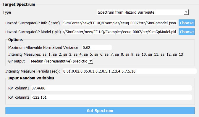
5. Once the above configurations are set up, click Get Spectrum button which will launch backend surrogate applications to predict the response spectrum at the provided location. Note although this example shows the application for predicting the response spectrum at a given location, the surrogate model can be trained on other input variables (not necessarily Longitude and Latitude).

6. Once the prediction is completed, the Target Spectrum widget will automatically switch to User Specified option with the tabulated response spectrum predicted for the given input variables.

3.7.3. Select Ground Motion and Run Analysis

1. Once the target response spectrum is available, users can follow the same procedure as introduced in EE-UQ Example 3 to select and scale ground motion records.

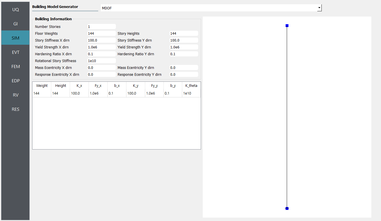
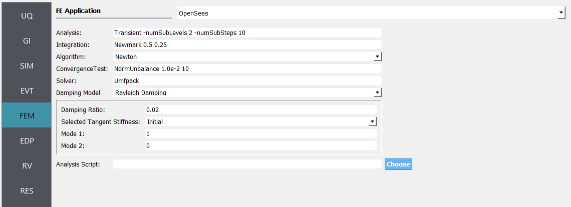
2. In the example, a simple SDOF model is used in SIM tab to demonstrate the structural analysis step and default configurations are used in the FEM and EDP tabs.

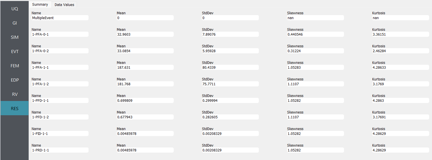
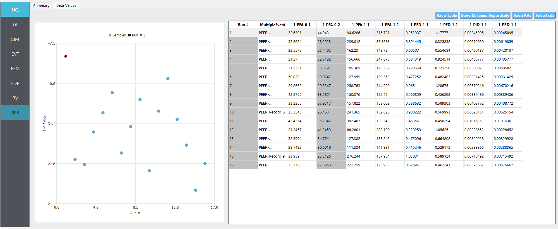
3. By clicking Run button, one can launch the analysis and the application will automatically switch to the RES tab once the analysis is completed. One could navigate to the Data Value panel to visualize and save the new realizations.