This example demonstrates Multi-fidelity Monte Carlo (MFMC) supported in EE-UQ. The high- and low-fidelity building models of a benchmark 9-story steel structure ([Ohtori2004]) are used for the demonstration, following the implementation in ([Patsialis2023]).
Fig. 4.11.1 Illustration of Multi-fidelity Monte Carlo
Patsialis, D., Taflanidis, A. A., & Vamvatsikos, D. (2023). Improving the computational efficiency of seismic building-performance assessment through reduced order modeling and multi-fidelity Monte Carlo techniques. Bulletin of Earthquake Engineering, 21(2), 811-847.
The target structure is a nine-story moment-resisting five-bay frame with a total height of 37.19 m and a length of 45.73 m.
The
High-Fidelity model (main script: benchmark_9st_model.tcl) is a nonlinear finite element model developed in OpenSees. Material characteristics are modulus of elasticity E=1.99 105 MPa for both beams and columns, yield stress for the columns 345 MPa and 248 MPa for the beams using values proposed in [Ohtori2004]. For modeling material inelastic behavior, the Giufre’-Menegotto-Pinto model with isotropic strain hardening is chosen for the steel fibers. The fundamental period is 2.274 sec, and under the Rayleigh damping assumption, the damping ratio is selected as 2% for the 1st and 3rd modes.
The Low-Fidelity model (main script: Alt_ROM_Simulation_BoucWen_Drift.tcl) is the reduced-order model (ROM) of the high-fidelity model. The detailed development procedures can be found in [Patsialis2020A] and [Patsialis2020B]. As promoted in the papers, the Bouc-Wen hysteretic model is chosen for the nonlinear connections of the ROM. The parameters of the ROM are chosen to minimize the error from the high-fidelity response, where three ground motion records are used to generate the reference high-fidelity prediction and optimize low-fidelity predictions.
In the example, the computation time of the low-fidelity model is expected to be 40-50 times faster than that of the high-fidelity model.
Patsialis D, Tafanidis AA (2020) Reduced order modeling of hysteretic structural response and applications to seismic risk assessment. Eng Struct 209:110135.
Patsialis D, Kyprioti AP, Tafanidis AA (2020) Bayesian calibration of hysteretic reduced order structural models for earthquake engineering applications. Eng Struct 224:111204
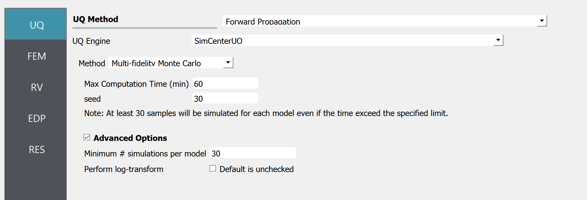
Let us set the maximum computation time to be 60 minutes. Random seed can be any positive integer and is only for reproducibility purposes. Check the Advanced Options and set the minimum number of simulations to 30. Additionally, the the statistics will be estimated in a log scale by checking perform log-transform check box.
Note
Note that the maximum computation time is a ‘soft’ target, rather than a hard time limit. The total number of simulations is decided after a few pilot simulations (# = 30 in this example) considering the remaining budgets (time), and the process is not enforced to finish even if the target time is exceeded. Therefore, there could be a few minutes of estimation error in the max computation time.
The GI tab is kept as default. (GI tab is not used when OpenSees models are imported in SIM tab)
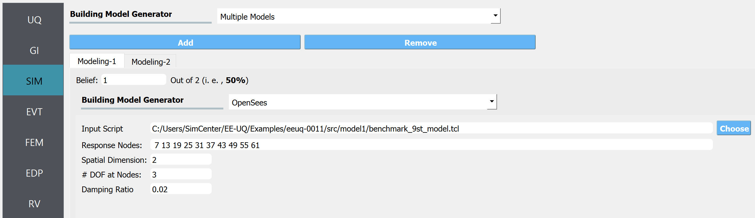
In SIM tab, select the Multiple Models option. Use Add button to import two models. The model with a lower index value should be a higher fidelity model. Therefore, high-fidelity and low-fidelity models should respectively be loaded in Model 1 and Model 2 tabs. In Model 1, import the main file, and set the response nodes by picking one node per story starting from the ground floor. In the current example, the ten nodes specified in the response nodes field, 7, 13, 19, 25, 31, 37, 43, 49, 55, 61, represent respectively from the ground floor(7) to the top story (61) ceiling. This is the list of nodes that will be used to evaluate the engineering demand parameters.
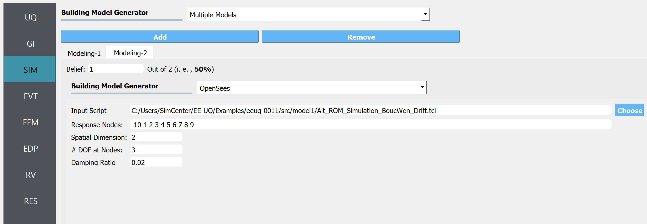
Similarly, the main analysis script for the low-fidelity model is imported into Model 2. The ten nodes specified in the response nodes field, 10, 1, 2, 3, 4, 5, 6, 7, 8, 9, represent respectively from the ground floor (10) to the top story (9) ceiling. This is again the list of nodes that will be used to evaluate the engineering demand parameters.
Both models have spatial dimensions of 2 and have 3 degrees of freedom per node.
Note
To run MFMC, it is important to make sure the two models have the exact same number of response nodes, and each of these nodes should have a one-to-one match between the two models.
Note
In case the structural models have uncertain parameters, MFMC requires the two models to share the same random variables as input. For example, if the floor height is the input random variable of the high-fidelity model, the low-fidelity model should also have the floor height as input. In this example, the structure is considered deterministic, and only the uncertainty in the ground motion model (moment magnitude and random time history) is considered.
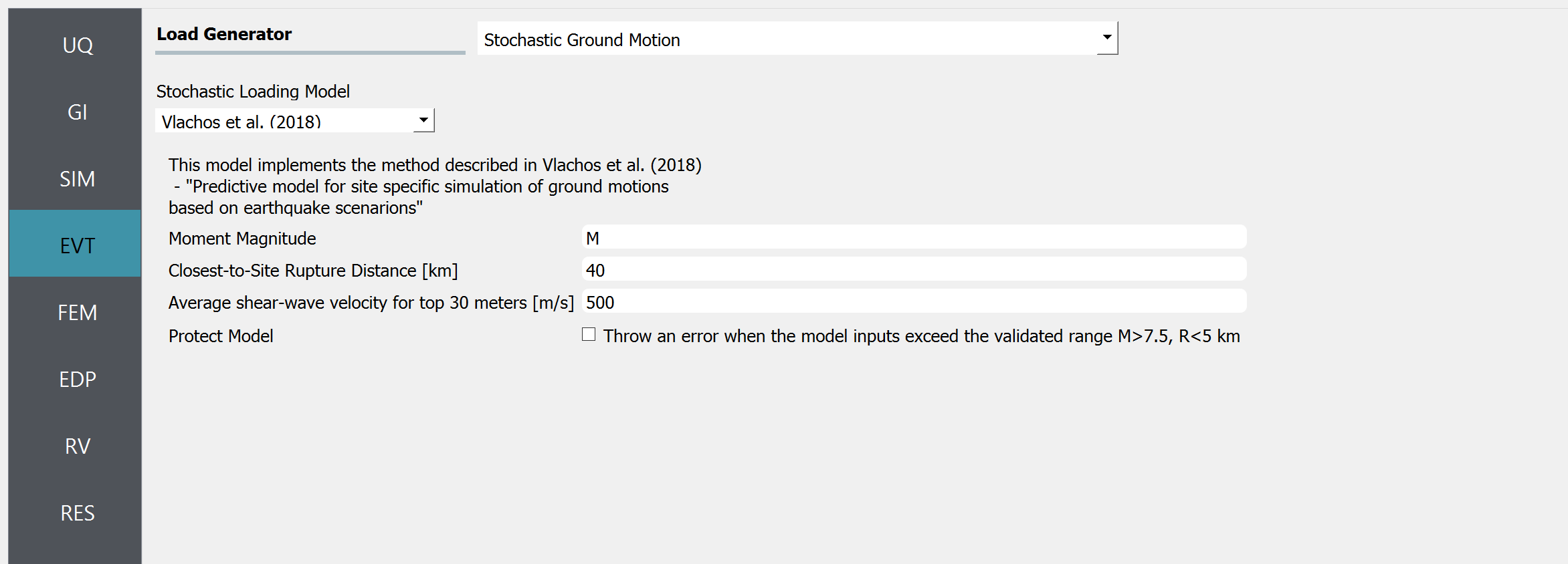
In EVT tab, Stochastic Ground Motion option is selected. In particular, Vlachos et al. (2018) is selected among alternatives. Let us assume the Moment Magnitude is a random variable by putting the letter M instead of a number. The random distribution can be specified later in the RV tab
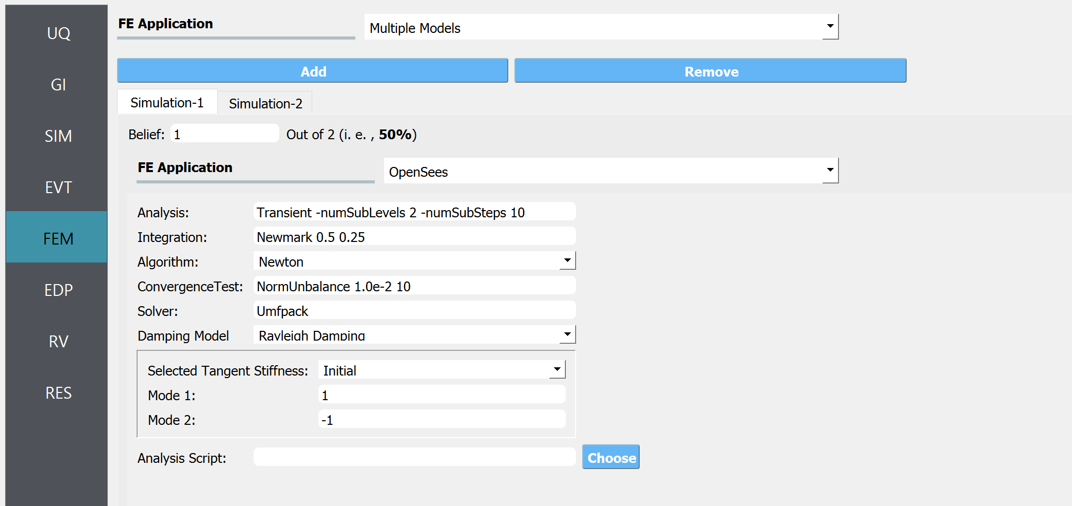
In FEM tab, Multiple Models are selected, similar to what was done for SIM tab. Each model in the FEM tab corresponds to that in the SIM tab. For the high-fidelity model, we will use the OpenSees FE application with the default options.
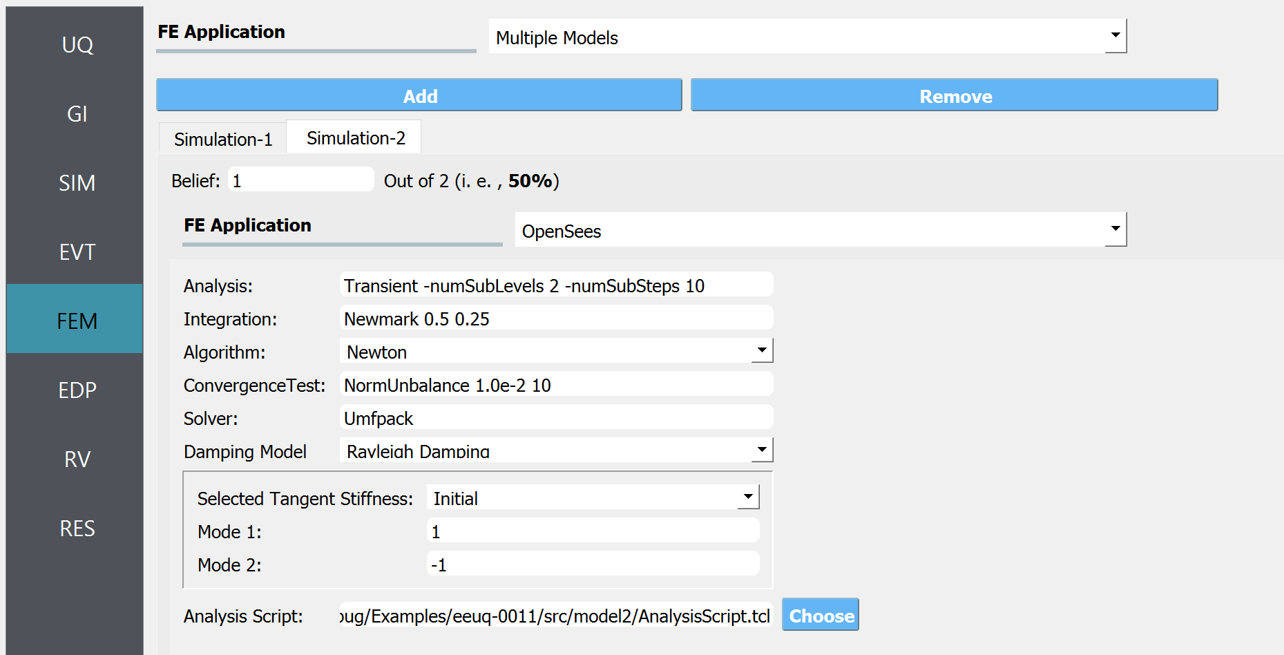
For the low-fidelity model, again select the OpenSees FE application. But to increase the stability of eigenvalue analysis, we will use a custom analysis script with an additional “-fullGenLapack” flag. Import the analysis script to the Analysis Script field. The other options in the widget (Analysis, integration, Algorithm, ConvergenceTest, Solver, Damping etc.) will be ignored.
The EDP tab standard earthquake option is selected.
Note
Standard Earthquake gives the repose values on each floor (Peak floor acceleration, peak floor displacement, peak inter-story drift), where the locations of floors are identified from the response node specified in the SIM tab as each floor. Notice that each of the 10 nodes we specified corresponds to the ground floor, first-floor ceiling, second-floor ceiling, …., and ninth-floor ceiling.
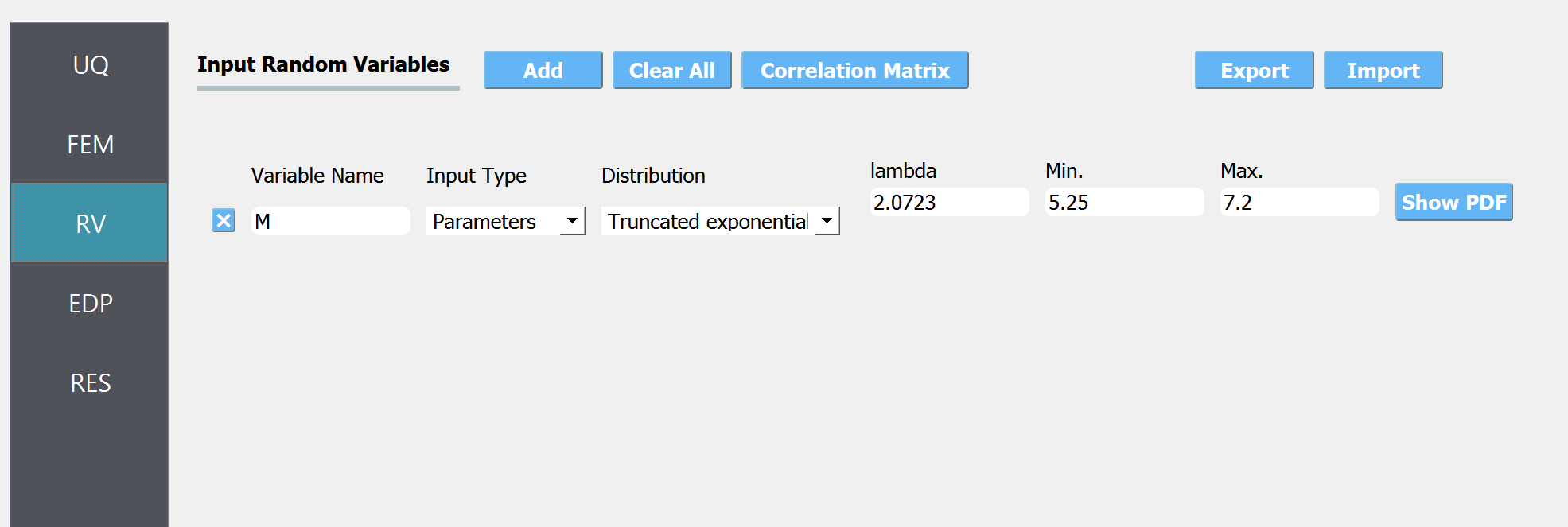
The RV tab is pre-populated with the variable M when we specified M in the EVT tab. Let us assume the Gutenberg-Richter model truncated in interval [6, 8], which lead to a truncated exponential distribution. The parameter of the distribution is taken to be \(0.9ln(10)=2.0723\).
Click Run button. The analysis may take several minutes. The RES tab will be highlighted when the analysis is completed
The EDP name consists of the quantity of interest, story number, and the direction of interest - for example:
1-PFA-0-1-M1 : peak floor acceleration at the ground floor, component 1 (x-dir), response from Model 1
1-PFD-1-2-M1 : peak floor displacement (respective to the ground) at the 1st floor ceiling, component 2 (y-dir), response from Model 1
1-PID-3-1-M2 : peak inter-story drift ratio of the 1st floor, component 1 (x-dir) , response from Model 2
1-PRD-1-1-M2 : peak roof drift ratio, component 1 (x-dir) , response from Model 2
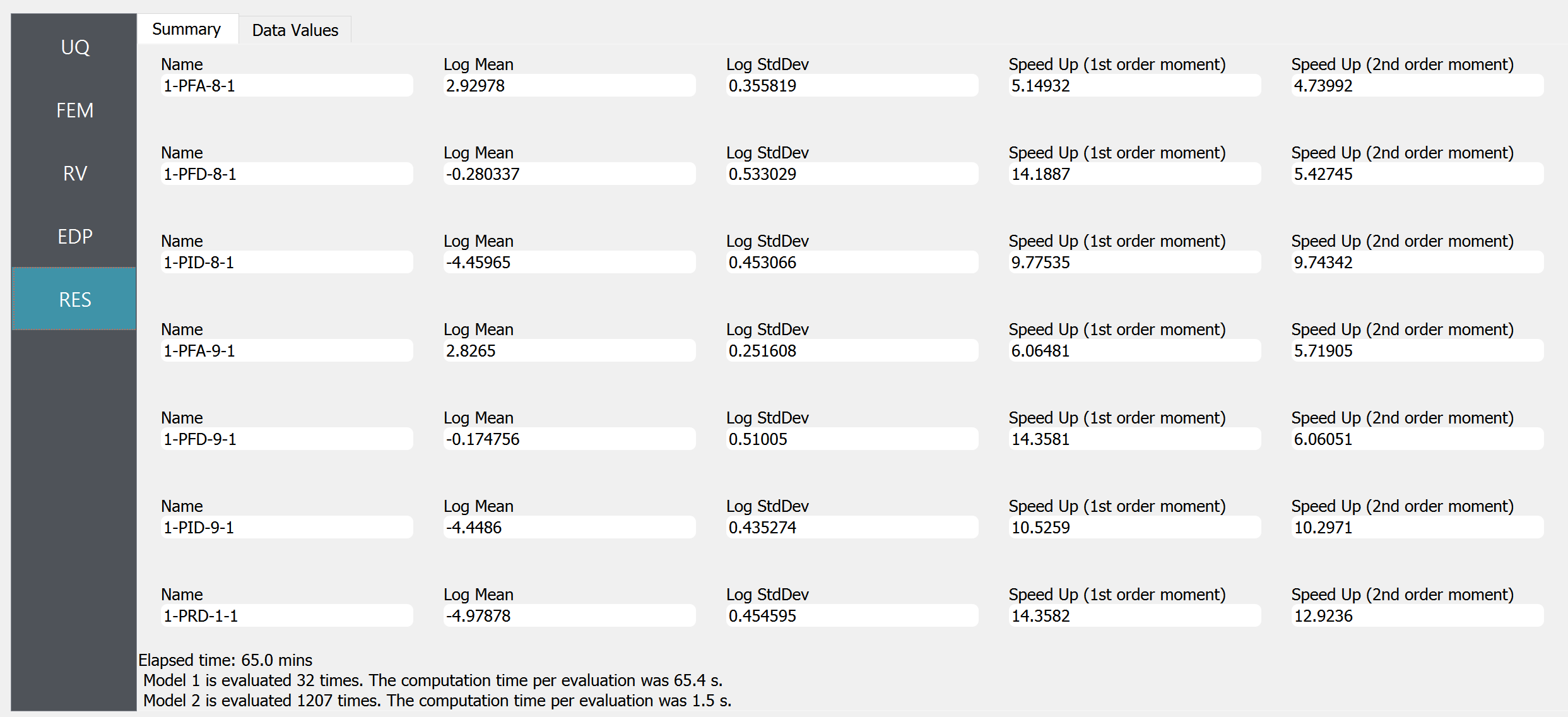
The obtained statistics of responses are shown in the “Summary tab”
Fig. 4.11.3.1 RES tab - summary of response statistics
The results additionally show Speed Up factors by comparing the total analysis time with the expected analysis time required to get the same precision of the estimator using only the high-fidelity simulations. Note that the elapsed analysis time (65 mins) exceeded the specified max computation time (60 mins) by 10% for the reasons explained earlier in this page. The computation time per model evaluation is “wall-clock” time, and because the example is computed using 8 processors, the actual analysis time of each model in a single processor is 8 times longer.
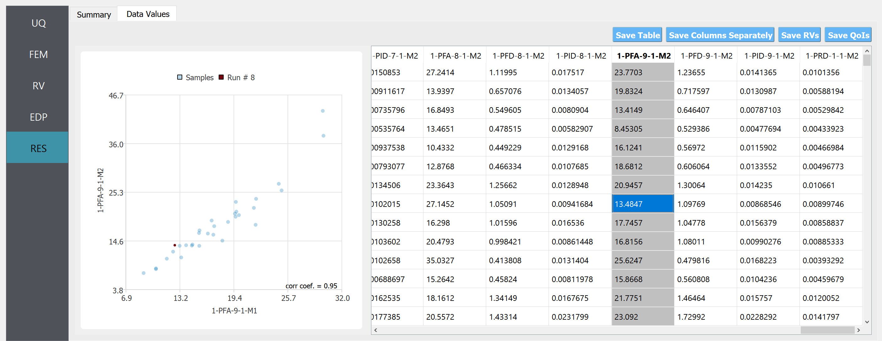
In the “Data Values” tab, one can plot the histogram and cumulative density function (CDF) of the samples, as well as scatter plots between the input and output of surrogate predictions. Using this feature, one can draw a scatter plot between low- and high-fidelity model responses. This is useful because it gives intuition on how informative the low-fidelity model run is.
Fig. 4.11.3.2 RES tab - cumulative density function
Note
The user can interact with the plot as follows.
Windows: left-click sets the Y axis (ordinate). right-click sets the X axis (abscissa).
MAC: fn-clink, option-click, and command-click all set the Y axis (ordinate). ctrl-click sets the X axis (abscissa).
4.11.4. Comparison to High-fidelity-only and low-fidelity-only simulations
Only for validation purposes, high-fidelity simulations are performed 1000 times and the resulting statistics (reference) are compared with the above multifidelity (MF) estimates. Recall that the estimation was based on 32 high-fidelity (HF) simulations and 1027 low-fidelity (LF) simulations.
Fig. 4.11.4.1 Error in MF, HF-only, and LF-only estimations of the first- and second-order moments. MF effectively reduces the sample variability observed in HF-only estimates and corrects the bias in LF-only estimates (Seed = 30).
The presented error (y-axis) is the absolute un-normalized difference between the reference and the estimated moments. Note that the large errors in HF results are attributed to sample variability originating from the small sample size. As more HF simulations are performed, HF error will approach zero. On the other hand, the errors in LF results are attributed to inherent bias, and therefore, it is not likely to be reduced by adding more samples. Meanwhile, MF results successfully correct the bias in the LF estimations, by additionally utilizing the 32 HF simulation samples. To emphasize the different nature of the errors observed in HF and LF estimates (i.e., the former representing sample variability and the latter representing inherent model bias), the Multi-fidelity Monte Carlo is performed once more with a different initial random seed (seed is specified in the UQ Tab). The corresponding validation results are presented below.
Fig. 4.11.4.2 Error in MF, HF, and LF estimations. MF reduces the sample variability observed in HF and corrects the bias in LF estimation (Seed = 3).
Note that the level of error observed in the LF model (green) is almost consistent in the two analyses, while HF error (orange) is highly dependent on the sample quality.