3.1. Sampling, Reliability and Sensitivity Analysis of a Shear Building

Consider the problem of uncertainty quantification for a three-story shear building

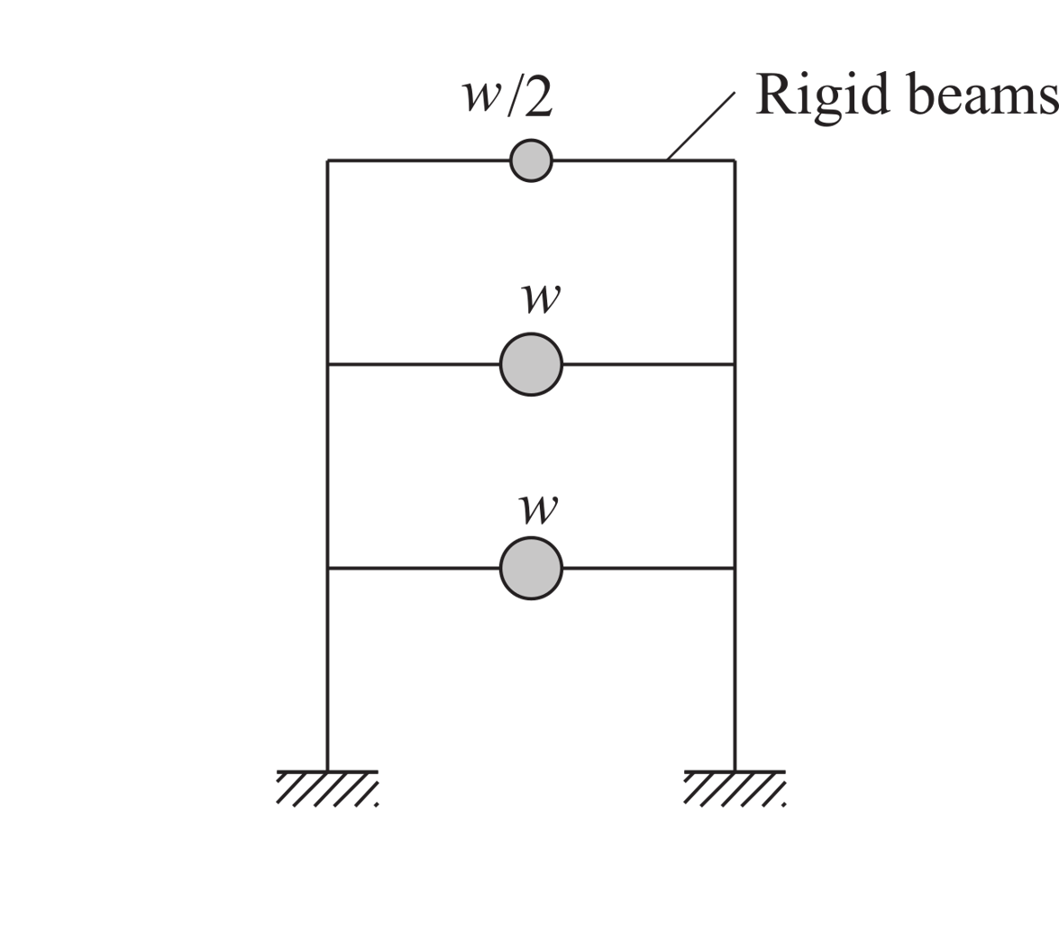
Fig. 3.1.1 Three Story Shear Building Model (P10.2.9, “Dynamics of Structures”, A.K.Chopra)

The structure has uncertain properties that all follow a normal distribution:

1. Weight of Typical Floor (w): mean \(\mu_E=100 \mathrm{kip}\) and standard deviation \(\sigma_E =10 \mathrm{kip}\) (COV = 10%)

2. Weight of Roof (wR): mean \(\mu_E=50 \mathrm{kip}\) and standard deviation \(\sigma_E =5 \mathrm{kip}\) (COV = 10%)

3. Story Stiffness (k): mean \(\mu_k =326.32 \mathrm{kip/in}\) and a standard deviation of \(\sigma_P = 3 \mathrm{kN}\), (COV = 12%).

The goal of the exercise is to estimate the mean and standard deviation of the relative displacement of the fourth node when subjected to an El Centro ground motion record.

The exercise will use both the MDOF, Multiple Degrees of Freedom (MDOF), and OpenSees, OpenSees, structural generators. For the OpenSees generator the following model script, ShearBuilding3.tcl , is used:

#units kips/in

# some parameters
# pset is used for set up random variables
pset w 100.0
pset wR 50.0
pset k 326.32

set E 29000.0
set A 1e4
set Ic [expr $k*144*144*144/(24.*$E)]
set Ib 1e12
set g 386.1

puts [expr $w/$g]
puts [expr $wR/$g]

# the model
model BasicBuilder -ndm 2 -ndf 3
# create node
# node $nodeTag $X $Y <-mass $massX $massY $massR>
node 1    0.   0.0 
node 2    0. 144.0 -mass [expr $w/$g] [expr $w/$g]     0.
node 3    0. 288.0 -mass [expr $w/$g] [expr $w/$g]     0.
node 4    0. 432.0 -mass [expr $wR/$g] [expr $wR/$g]   0.
node 5  288.   0.0 
node 6  288. 144.0 
node 7  288. 288.0 
node 8  288. 432.0 
# boundary conditions
# fix $nodeTag $bcX $bcY $bcR
fix 1 1 1 1
fix 5 1 1 1
# constrain nodal DOFs
# equalDOF $nodeTag1 $nodeTag2 $DOF
equalDOF 2 6 1
equalDOF 3 7 1
equalDOF 4 8 1
# geometric transformation
# geomTraf $type $tranfTag
geomTransf Linear 1
# element elasticBeamColumn $elementTag $nodeTag1 $nodeTag2 $area $momentOfInertia $modulus $tranfTag
element elasticBeamColumn 1 1 2 $A $Ic $E 1
element elasticBeamColumn 2 2 3 $A $Ic $E 1
element elasticBeamColumn 3 3 4 $A $Ic $E 1
element elasticBeamColumn 4 5 6 $A $Ic $E 1
element elasticBeamColumn 5 6 7 $A $Ic $E 1
element elasticBeamColumn 6 7 8 $A $Ic $E 1
element elasticBeamColumn 7 2 6 $A $Ib $E 1
element elasticBeamColumn 8 3 7 $A $Ib $E 1
element elasticBeamColumn 9 4 8 $A $Ib $E 1

Note

1. The first lines containing pset will be read by the application when the file is selected and the application will autopopulate the random variables w, wR, and k in the RV panel with these same variable names.

Warning

Do not place the file in your root, downloads, or desktop folder as when the application runs it will copy the contents on the directories and subdirectories containing this file multiple times (a copy will be made for each sample specified). If you are like us, your root, Downloads or Documents folders contain and awful lot of files and when the backend workflow runs you will slowly find you will run out of disk space!

3.1.1. Sampling Analysis with El Centro

We will first demonstrate the steps to perform a sampling analysis to study the effects of the roof response of models of the building subjected to the El Centro ground motion. We will scale the input motion using a scale factor (which we name factorEC) following a uniform distribution between 1.2 and 1.8, i.e. mean \(\mu_{factorEC} = 1.5\) and a standard deviation of \(\sigma_{factorEC} = 0.1732\), (COV = 12%).

To perform a Sampling or Forward propagation uncertainty analysis the user would perform the following steps:

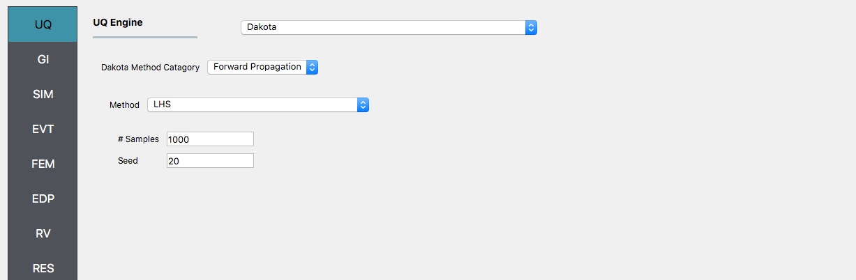
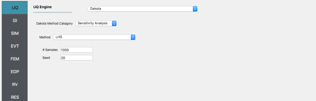
1. Upon opening the application the UQ tab will be highlighted. In is panel, keep the UQ engine as that selected, i.e. Dakota, and the UQ Method Category as Forward Propagation, and the Method field as LHS (Latin Hypercube). Change the #samples field to 1000 and the Seed to 20 as shown in the following figure.

Note

When loading the example from the tool page, the number of samples is set to 50.

2. The GI panel will not be used for this run; For the time being leave the default values as is, and they will be automatically updated based on the information entered in the remaining tabs.

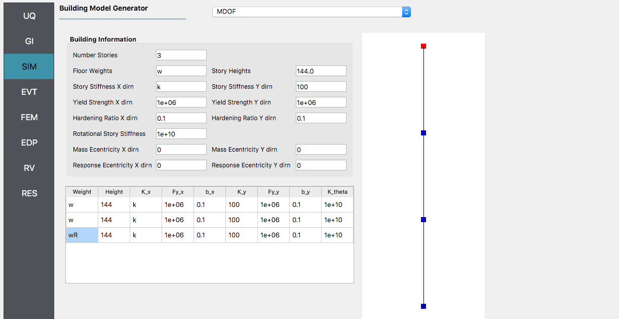
3. Next select the SIM panel from the input panel. This will default in the MDOF model generator. We will use this generator (the NOTE below contains instructions on how to use the OpenSees script instead). In the building information panel, specify the number of stories as 3 (this will change the graphic). Also in the Building information frame specify w for the floor weights and k for story stiffness. Finally, in the table below, go to the third row and enter wR for the roof weight (you will notice that when you enter that table cell the node at the top of the model will turn red, indicating you are editing the information for the top most node).

Note

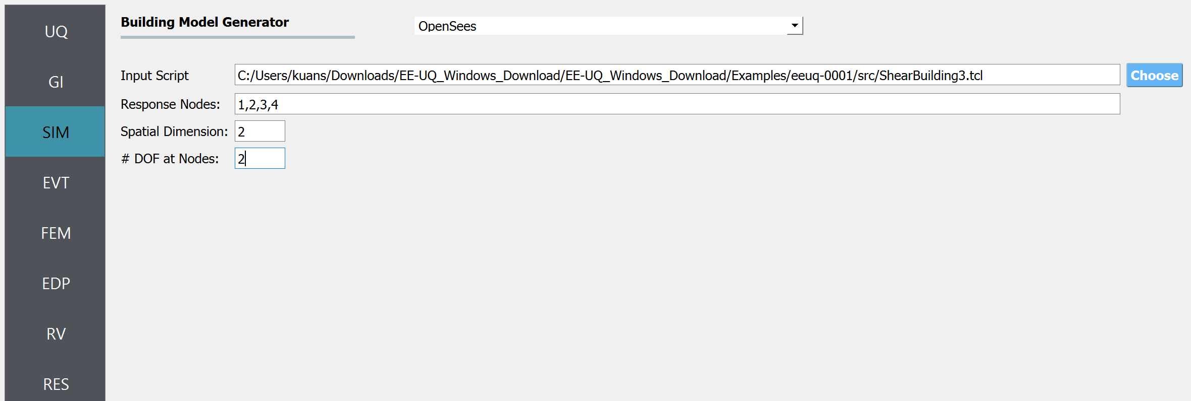
To specify instead to use the OpenSees script, from the Model Generator pull-down menu select OpenSees. For the fields in the panel presented enter the path to the ShearBuilding3d.tcl script. Also, specify three Response Nodes as 1 2 3 4 in the panel. This field will tell the model generator which nodes correspond to nodes at the four-floor levels at which responses are to be obtained when using the standard earthquake EDPs.

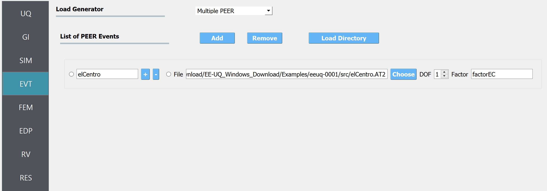
4. Next select the EVT panel. From the Load Generator pull-down menu select the Multiple PEER option. This will present a panel with three buttons: Add, Remove and Load Directory. Click the Add button. Give the motion a name, here enter elCentro in the first line edit. Now for the motion, enter the path to the elCentro.AT2 motion. Leave the motion acting in the 1 dof direction and for the scale factor in this direction, enter factorEC.

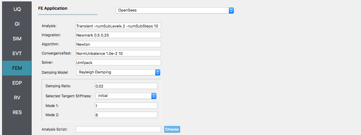
5. Next choose the FEM panel. Here we will change the entries to use Rayleigh damping, with Rayleigh factor chosen using the first and third modes. For the MDOF model generator, because it generates a model with two translational and one rotational degree-of-freedom in each direction and because we have provided the same k values in each translational direction (i.e. we will have duplicate eigenvalues), we specify as shown in the figure modes 1 and 6.

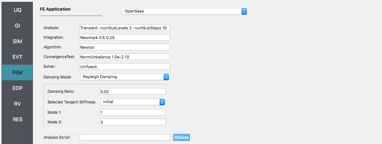
Note

If instead we were using the OpenSees model, which does not have the duplicate eigenvalues, it being a planar problem with constrained degrees-of-freedom, we specify modes 1 and 3 as shown.

6. We will skip the EDP panel leaving it in its default condition, that is to use the Standard Earthquake EDP generator.

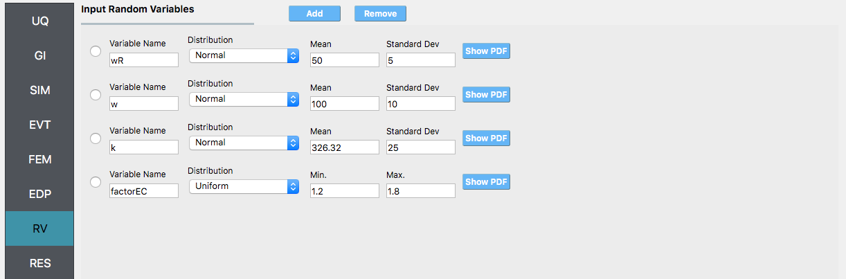
7. For the RV panel, we will enter the distributions and values for our random variables. Because of the steps we have followed and entries we have made, when this tab is opened it should contain the four random variables and they should all be set constant. For the w, wR and k random variables we change the distributions to normal and enter the values given for the problem, as shown in the figure below. For the factorEC variable, change the distribution to uniform and enter the values in the figure.

Warning

The user cannot leave any of the distributions for these values as constant for the Dakota UQ engine.

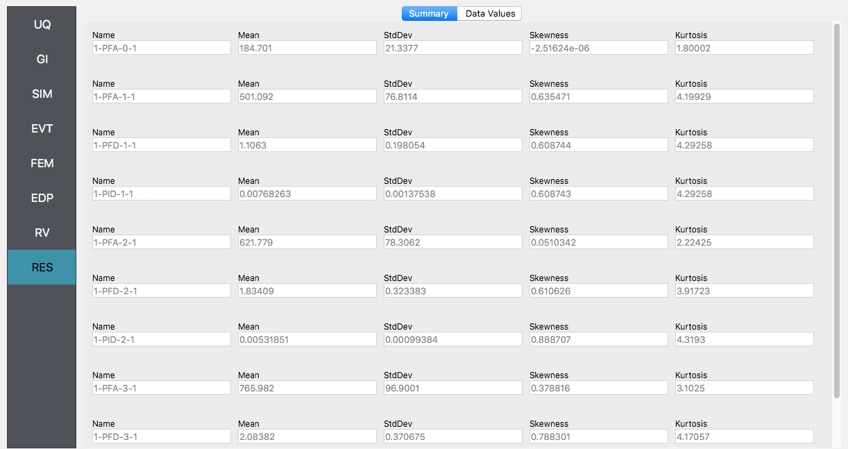
8. Next click on the Run button. This will cause the backend application to launch Dakota. When the analysis is complete the RES tab will be selected and the results will be displayed. The results show the values for the mean and standard deviation. The relative displacement of the roof is the quantity 1-PFD-3-1. This identifier signifies the first event, 3rd floor (in the US the ground floor is considered 0), and the first dof direction.

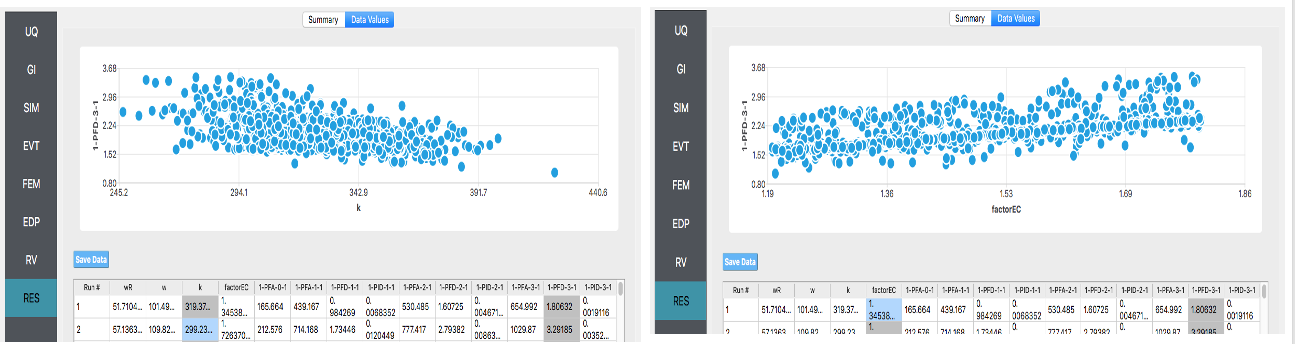
If the user selects the Data tab in the RES panel, they will be presented with both a graphical plot and a tabular listing of the data. By left- and right-clicking with the mouse in the individual columns the axis changes (the left mouse click controls the vertical axis, right mouse clicks the horizontal axis).

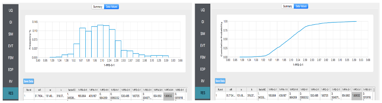
Various views of the graphical display can be obtained by left- and right-clicking in the columns of the tabular data. If a singular column of the tabular data is selected with both right and left mouse buttons, a frequency and CDF plot will be displayed, as shown in the figure below.

3.1.2. Sampling Analysis with ElCentro and Reduced Output

In the previous example, we got the standard output, which can be both a lot and also limited (in the sense you don’t get the information you want). In this example we will present how to obtain results just for the roof displacement, the displacement of node 4 in both the MDOF and OpenSees model generator examples. The examples could be extended to output for example the story shear forces, element forces, element end rotations, etc.

For this example, you will need two additional files recorderCommands.tcl and postprocess.tcl. The recorderCommands.tcl script as shown below will record the envelope displacements in the first two degrees of freedom for nodes 1 through 4.

recorder EnvelopeNode -file node.out -node 1 2 3 4 -dof 1 2 disp
recorder EnvelopeElement -file forces.out -ele 1 2 3 forces

The postprocess.tcl script shown below will accept as input any of the 4 nodes *in the domain and for each of the two dof directions.

set nodeIn [open node.out r]
while { [gets $nodeIn data] >= 0 } {
     set maxDisplacement $data
}
puts $maxDisplacement

# create file handler to write results to output & list into which we will put results
set resultFile [open results.out w]
set results []

# for each quanity in list of QoI passed
#  - get nodeTag
#  - get nodal displacement if valid node, output 0.0 if not
#  - for valid node output displacement, note if dof not provided output 1'st dof

foreach edp $listQoI {
	set splitEDP [split $edp "_"]	
	set nodeTag [lindex $splitEDP 1]
        if {[llength $splitEDP] == 3} {
           set dof 1
	} else {
            set dof [lindex $splitEDP 3]
	} 
    set nodeDisp [lindex $maxDisplacement [expr (($nodeTag-1)*2)+$dof-1]]
	lappend results $nodeDisp
}

# send results to output file & close the file
puts $resultFile $results
close $resultFile

Note

The user has the option to provide no postprocess script (in which case the main script must create a results.out file containing a single line with as many space-separated numbers as QoI or the user may provide a Python script that also performs the postprocessing. An example of a postprocessing Python script is postprocess.py.

The steps are the same as the previous example, with the exception of step 4 defining the EDP. 5.

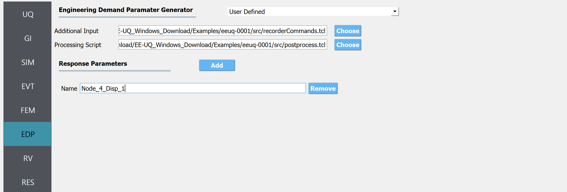
1. For the EDP panel, we will change the generator to User Defined. In the panel that presents itself, the user must provide the paths to both the recorder commands and the postprocessing script. Next, the user must provide information on the response parameters they are interested in. The user presses the Add button and enters Node_4_Disp_1 in the entry field as shown in the figure below.

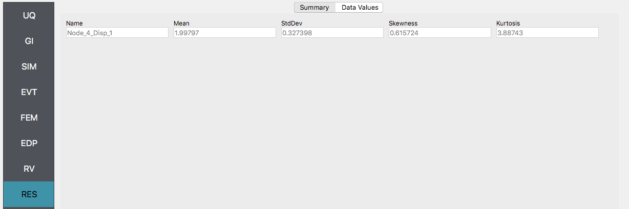
2. Next click on the Run button. This will cause the backend application to launch dakota. When done the RES panel will be selected and the results will be displayed. The results show the values of the mean and standard deviation as before but now only for the one quantity of interest.

3.1.3. Global Sensitivity

In a global sensitivity analysis, the user wishes to understand what is the influence of the individual random variables on the quantities of interest. This is typically done before the user launches large-scale forward uncertainty problems in order to limit the number of random variables used so as to limit the number of simulations performed.

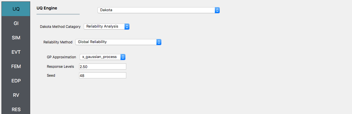
To perform a reliability analysis, the steps above would be repeated with the exception that the user would select a reliability analysis method instead of a Forward Propagation method. To obtain reliability results using the global reliability method for this problem the user would follow the same sequence of steps as previously. The difference would be in the UQ panel in which the user would select a Reliability as the Dakota Method Category and then choose GLobal reliability. In the figure, the user is specifying that they are interested in the probability that the displacement will exceed certain response levels.

After the user fills in the rest of the tabs as per the previous section, the user would then press the RUN button. The application (after spinning for a while with the wheel of death) will present the user with the results.

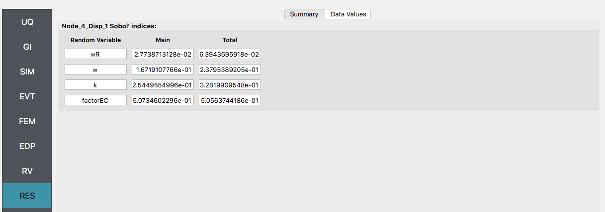
The results showing that the earthquake factor has the largest influence on the response followed by the stiffness value k, as the results graphically would indicate.

3.1.4. Reliability Analysis

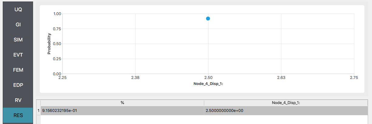
If the user is interested in the probability that certain response measures will be exceeded an alternative strategy is to perform a reliability analysis. To perform a reliability analysis the steps above would be repeated with the exception that the user would select a reliability analysis method instead of a Forward Propagation method. To obtain reliability results using the Global Reliability method presented in Dakota choose the Global Reliability methods from the methods drop-down menu. In the response levels enter a value of 2.5, specifying that we are interested in the value of the CDF for a displacement of the roof of 2.5in, i.e. what is the probability that displacement will be less than 2.5in.

After the user fills in the rest of the tabs as per the previous section, the user would then press the RUN button. The application (after spinning for a while with the wheel of death) will present the user with the results, which as shown below, indicate that the probability is 91.5%.

Warning

Reliability analysis can only be performed when there is only one EDP.