3.9. Training a Surrogate Model (Gaussian Process)

Warning

To reproduce the result of this example, the user should first click EVT and Select Records, and then click the RUN button. See the below procedure for details.

3.9.1. Training Gaussian Process Surrogate Model

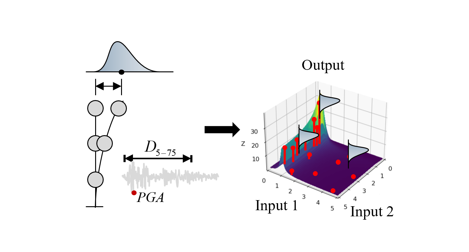
This example shows how to train a surrogate model that can be imported into EE-UQ and replace structural dynamic simulations. The training of a surrogate model requires some number of structural dynamic simulations for representative scenarios [i.e. training set]. In this example, these simulations are performed using recorded ground motions selected from the PEER NGA database. The ground motions are selected such that it covers a wide domain of intensity measure (IM) space, as uniform as possible. Three IMs are considered in the example: pseudo-spectral acceleration at period 0.5 sec (PSA), 5-75% duration (D5-75), and SaRatio following the work in [Zhong2023]. We additionally consider the stiffness of the target structure (3 story building) as input for the surrogate model.

Fig. 3.9.1.1 Training a surrogate model for seismic response

Zhong2023

Zhong, K., Navarro, J.G., Govindjee, S., and Deierlein, G.G., “Surrogate Modeling of Structural Seismic Response Using Probabilistic Learning on Manifolds,” Earthquake Engineering & Structural Dynamics, 1-22, (2023) https://doi.org/10.1002/eqe.3839

3.9.2. Set Up GP Surrogate Modeling Options

1. In the UQ tab select the Surrogate Modeling as UQ Method. Then, select the Train GP Surrogate Model.

   

   Fig. 3.9.2.1 UQ tab

   Below are the details of the selected inputs:

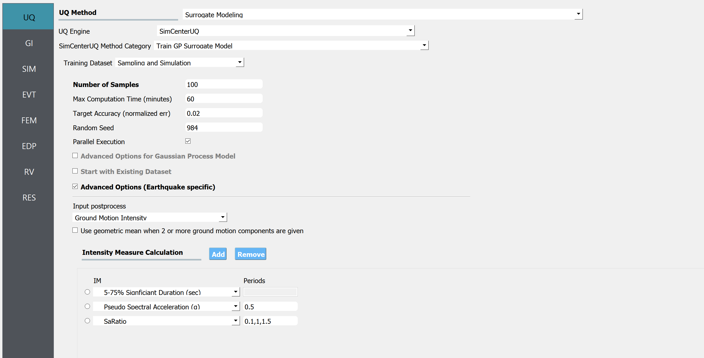
   • Number of Samples : The number of samples should be the same as the ground motions to be selected in the EVT tab, i.e. 100. This number can be flexible when stochastic ground motion is used. Typically, as the number of samples increases, the accuracy of the surrogate model will increase but training time will also increase.

   • Max Computation Time : 60 mins (default)

   • Target Accuracy : 0.02. EE-UQ will give a warning when this accuracy target is not met

   • Random Seed : 984. An arbitrarily selected seed for the random generator used in the Surrogate modeling algorithm

   • Parallel Execution : True. This will parallelize multiple dynamic simulations

   • Advanced Options for Gaussian Process Model : False. By default, EE-UQ takes Martern 5/2, Log-space transform of QoI, Heteroskedastic nugget variance options.

   • Existing Data set : False. This is useful when one hopes to resume the surrogate model training after one training round is finished, by performing more simulations

   • Intensity Measure Calculation: Select the intensity measures (IMs) to be used as the augmented input of the surrogate model -Sa(T=0.5 sec), D5-75, and SaRatio(T=1.0 sec in the range of 0.1-1.5 sec)

More information can be found in the User Guide.

3.9.3. Define Target Structure

1. In GI tab, set the number of stories, 3.

   

   Fig. 3.9.3.1 GI tab - Specify 3 story building

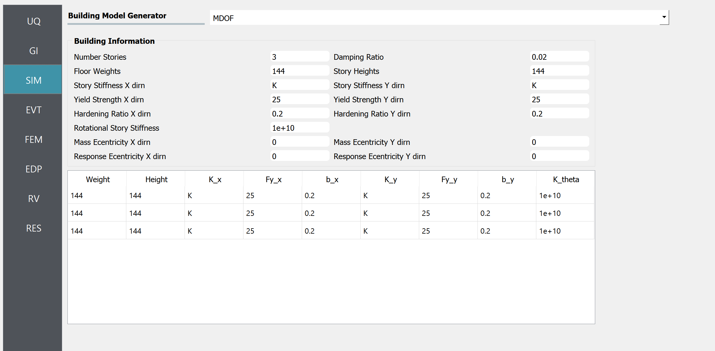
2. In SIM tab, the specifics of the target structural model is provided via MDOF building generator. A three-story building is created having stiffness as an input parameter.

   

   Fig. 3.9.3.2 SIM tab

3.9.4. Select Ground Motions for the Training

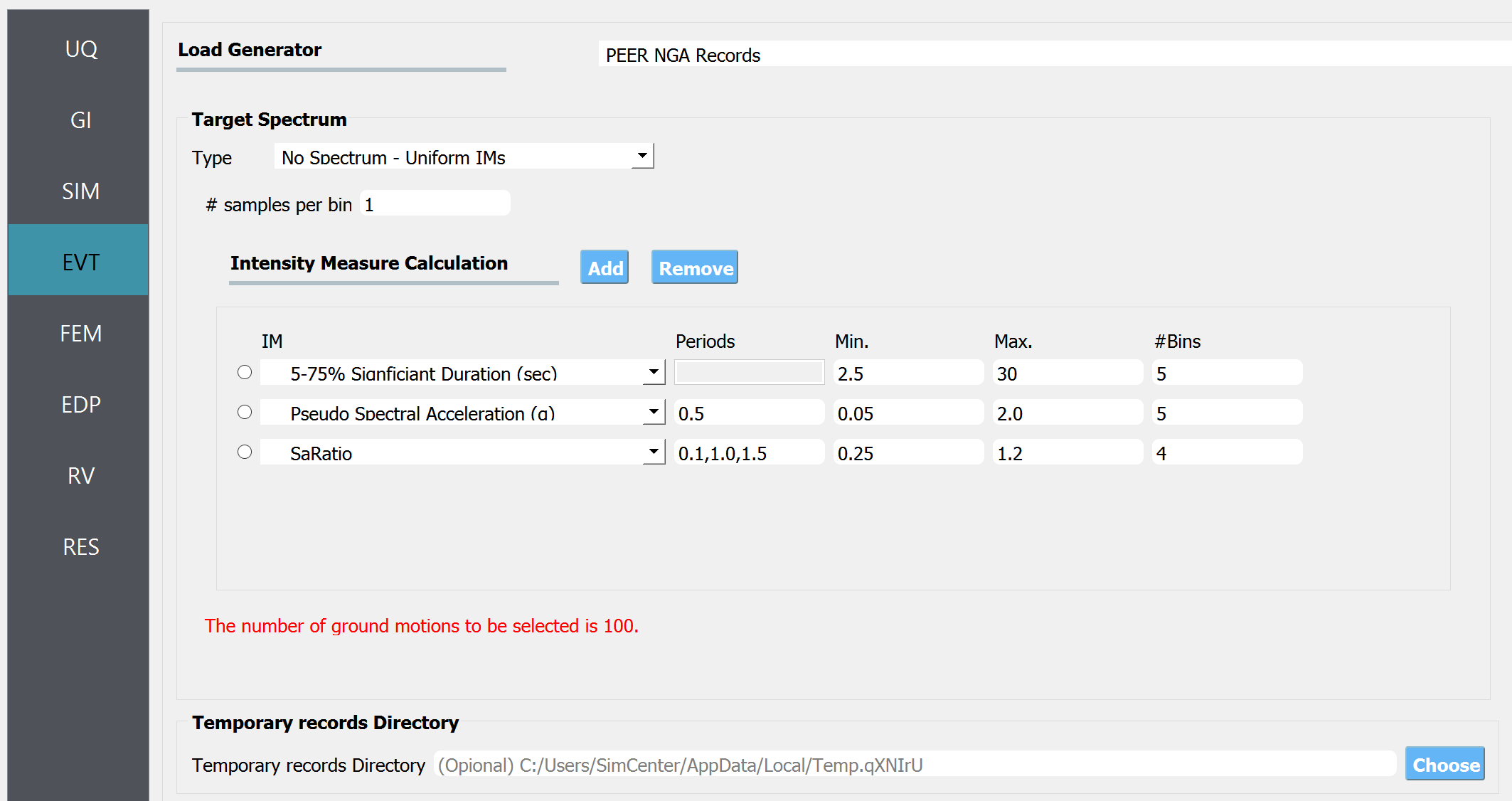
3. In EVT tab, the option to retrieve ground motions from PEER NGA records is selected. To allow the surrogate models to cover a wide variety of ground motions (represented as “wide IM domain”), let us select No Spectrum - Uniform IMs for the analysis. Set the Number of samples per bin 1, and add three intensity measures that are specified in the UQ tab as the input of surrogate, i.e. “5-75% Significant Duration”, “Pseudo Spectral Acceleration (with a natural period of 0.5 sec)”, and “SaRatio (at 1.0 sec in range of 0.1-1.5 sec). Set the coverage ranges respectively to [2.5, 30], [0.1, 2.0], and [0.25, 1.2]. For the former two IMs, the number of bins is set as 5, and the SaRatio will have 4 bins. Therefore, the total number of bins (i.e. grid points in 3-dimensional space) is 100.

   

   Fig. 3.9.4.1 EVT tab - configuration of IM bins

The selected excitation time histories will be saved in the “Temporary records Directory” shown in the figure. It is recommended to use a user-defined directory to reuse the data files in different analyses.

Warning

Due to copyright issues, PEER imposes a strict limit on the number of records that can be downloaded within a unique time window. The current limit is set at approximately 200 records every two weeks, 400 every month. Please make sure this limit is not exceeded. Otherwise, the analysis will fail.

• Temporary Records Directory is where the downloaded ground motion records are stored.

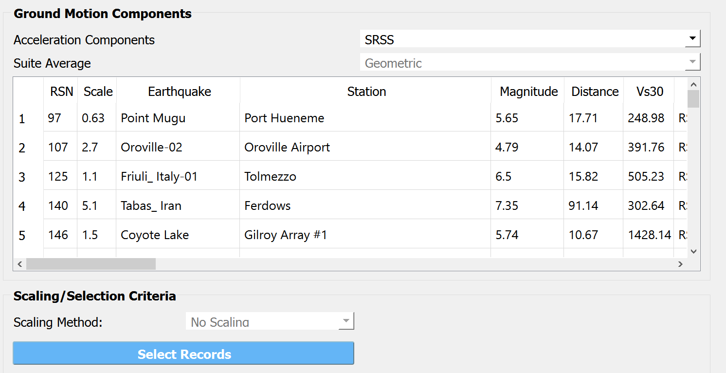
• Acceleration Components option is used to select the directional components to be used in the analysis. For example, if H1 is selected, single-directional ground motions will be excited to the structure.

  

  Fig. 3.9.4.2 EVT tab - Selected ground motions in a table

• Press Select Records when ready, which will connect the PEER NGA West Ground Motion Database. You could use your account and password to log in. If you don’t have an account, you can easily sign up at PEER Ground Motion Database. The list of selected ground motions and their scaling factors are displayed in the table. The coverage of IMs of the selected ground motions will be displayed in the right-hand side panel as below.

  

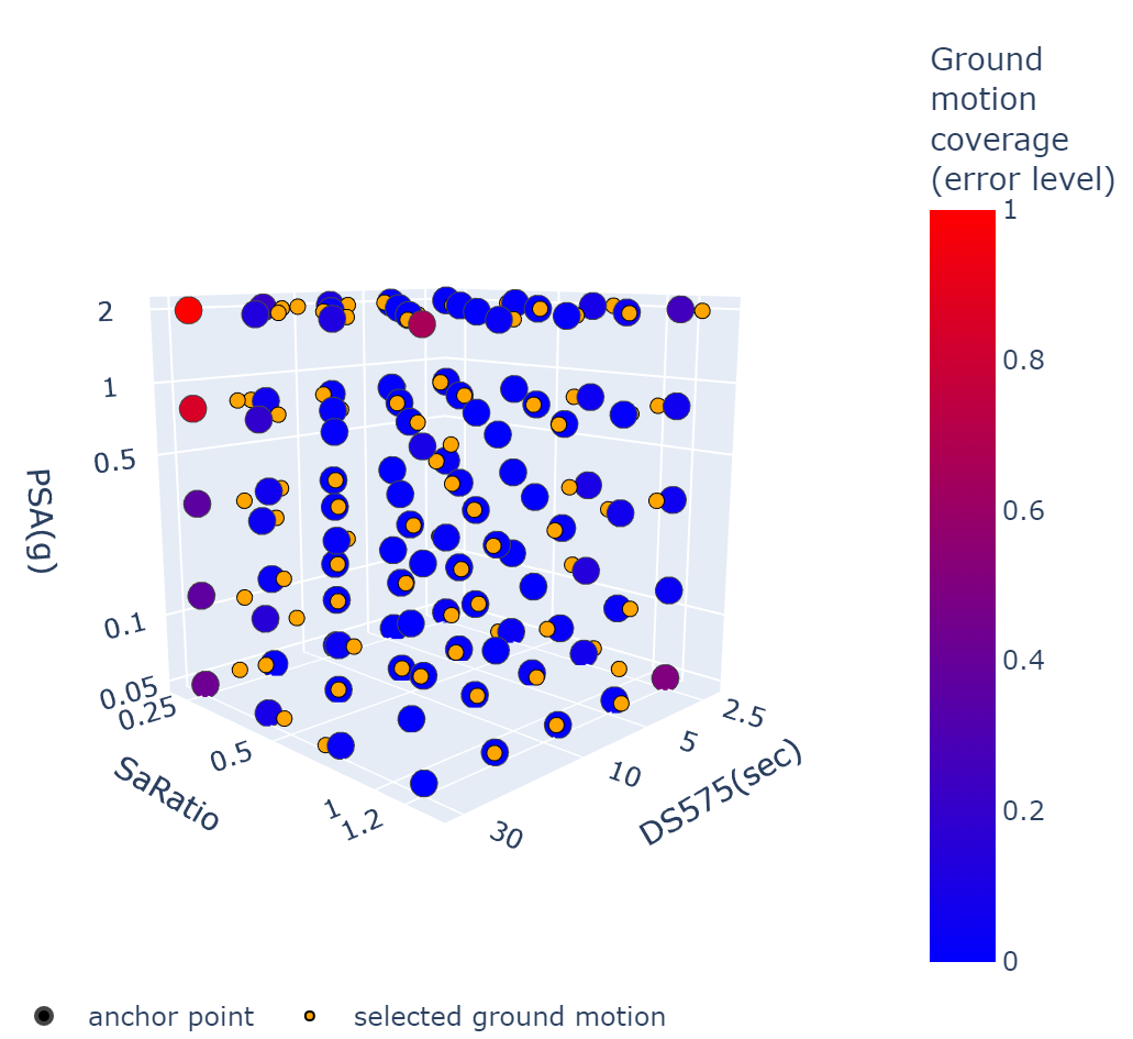
  Fig. 3.9.4.3 EVT tab - Selected ground motions in IM space

Note that approximated IM values are used for this ground motion selection. The approximated IMs are read from the flat file PEER provides, and the geometric mean is used to average out the two horizontal directional components. Therefore the actual IM used as the surrogate input may not exactly match the IM value shown in the above figure. The yellow dots represent the selected 100 ground motion records having corresponding IMs, blue/red dots represent the center of each bin, i.e. anchor point. It is colored red when no matching ground motion is found to be close to the anchor point. This informs users how good the IM coverage is.

Warning

Note that the surrogate modeling algorithms are stronger in “interpolation” rather than extrapolation. Therefore, when later using the pre-trained surrogate model to predict the response of the structure subjected to new (untrained) IM values (e.g. example 10), it is important to make sure the IMs of the new ground motions are well covered by the domain of the training samples, i.e. it should lie the area that is shown blue in the above figure. Otherwise, the prediction from the surrogate model is likely not reliable.

4. The FEM tab is kept as default.

Warning

Do NOT select the “None (only for the surrogate)” option in the FEM tab. This option is not for training a surrogate model but for using a pre-trained surrogate model. (See example 10)

5. The EDP tab is kept as default. For the surrogate model to be compatible with the PBE and other applications, it should follow the naming of the Standard Earthquake. Under the Standard Earthquake, in this example, the structural model will automatically output peak floor acceleration (PFA), peak floor displacement respective to the ground (PFD), Peak inter-story drift ratio (PID), peak roof drift ratio (PRD).

Warning

Do NOT select the “None (only for the surrogate)” option in the EDP tab. This option is not for training a surrogate model but for using a pre-trained surrogate model. (See example 10)

3.9.5. Set Up Training Domain

1. In RV tab set the range of stiffness to be [50, 150] as shown in the below image. This is equivalent to the range of stiffness of which the response can be predicted using the surrogate. The selected IMs (Sa, D5-75, and SaRatio) in each two horizontal directions will be additional inputs of the surrogate model. Therefore, the total dimension of the surrogate model input is 7.

   

   Fig. 3.9.5.1 RV tab

3.9.6. Run the Analysis and Process Results

6. Click Run button. The analysis may take several minutes to run. The RES tab will be highlighted when the analysis is completed.

   The EDP name consists of the quantity of interest, story number, and the direction of interest - for example:

   • 1-PFA-0-1 : peak floor acceleration at the ground floor, component 1 (x-dir)

   • 1-PFD-1-2 : peak floor displacement (respective to the ground) at the 1st floor ceiling, component 2 (y-dir)

   • 1-PID-3-1 : peak inter-story drift ratio of the 3rd floor, component 1 (x-dir)

   • 1-PRD-1-1 : peak roof drift ratio, component 1 (x-dir)

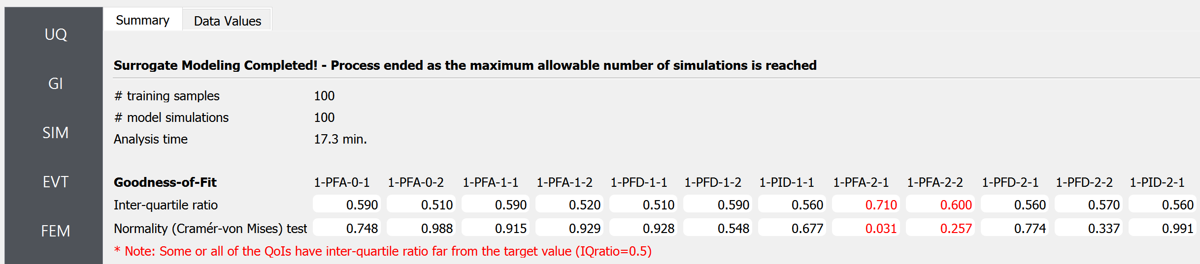
7. Two Goodness-of-fit measures are provided : Inter-quartile ratio (IQR) and normality (Cramer-Von Mises test) score. Using the leave-one-out cross-validation predictions, the IQR provides the ratio of the sample QoIs that lies in 25-75% LOOCV prediction bounds (interquartile range). The IQR values should theoretically approach 0.5 if the prediction is accurate.

   

   Fig. 3.9.6.1 RES tab - summary

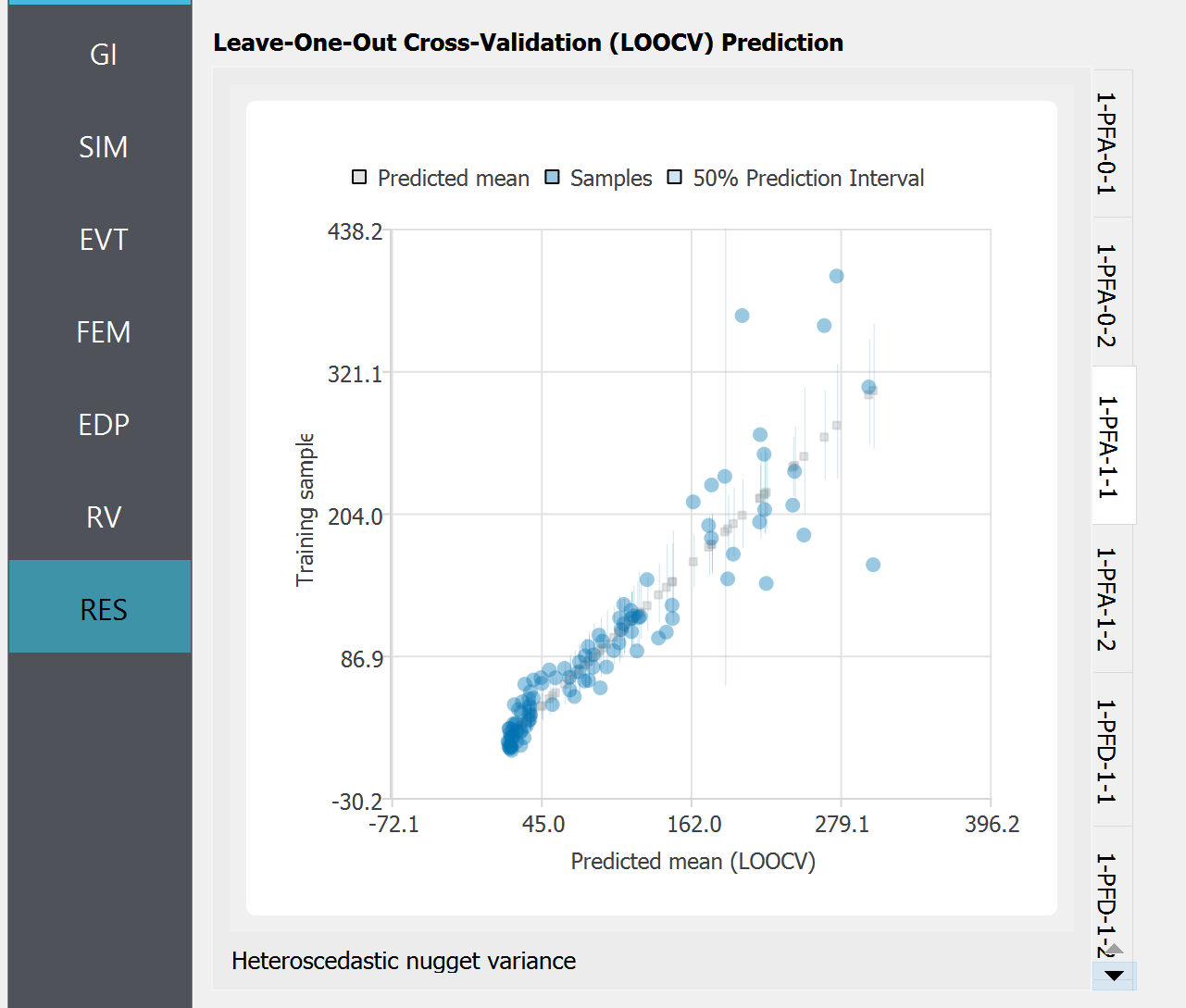
8. Additionally the comparison between the original simulation samples and leave-one-out cross-validation (LOOCV) predictions from the surrogate is provided as the scatter plot. When we have a large variance in the response observations, as in this example, the LOOCV mean is not expected to match exactly the data samples observed. Instead, they are expected to lie on a reasonable prediction bound. The below graph shows the inter-quartile prediction bounds, i.e. 25%-75%, which are expected to cover 50% of the sample observations.

   

   Fig. 3.9.6.2 RES tab - Leave-one-out cross-validation error measure

Please see the User Guide for more details on the verification measures.

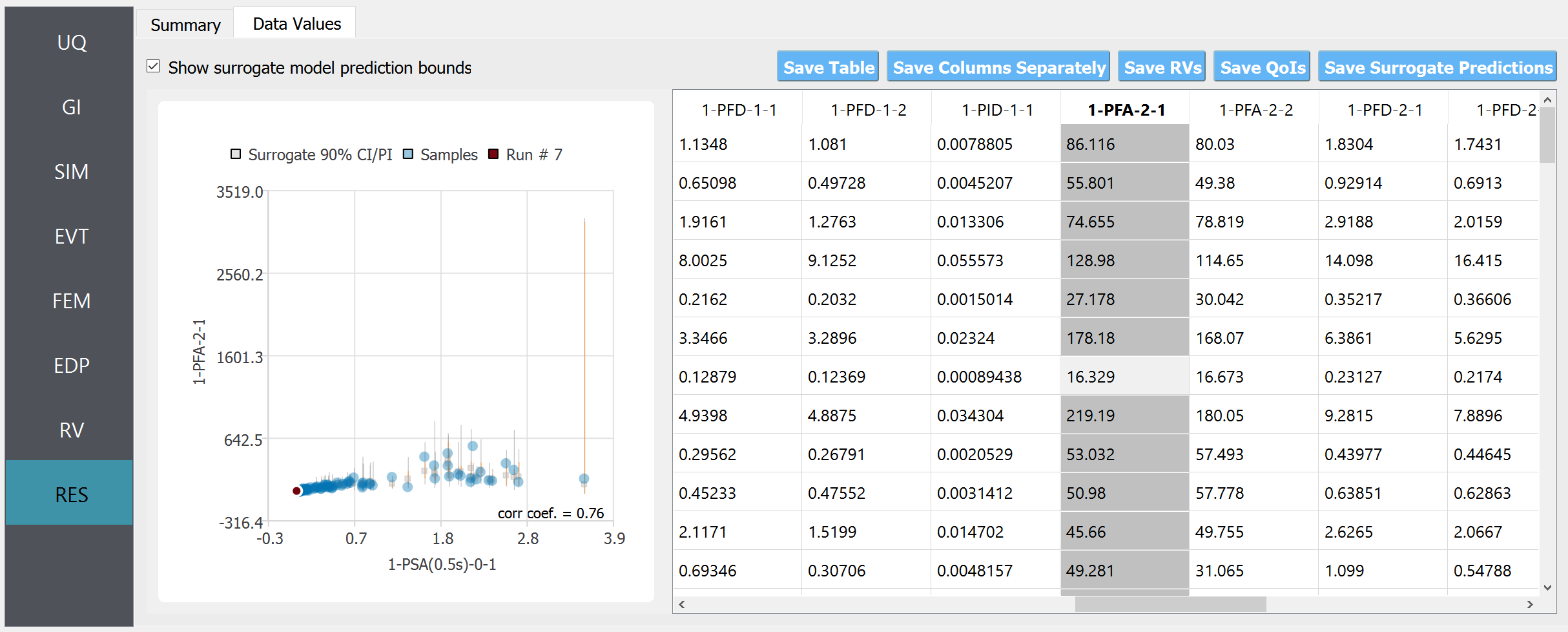
9. The LOOCV predictions can be compared for different input realizations under “Data Values” tab.

   

   Fig. 3.9.6.3 RES tab - Scatter plots

   Note

   The user can interact with the plot as follows.

   • Windows: left-click sets the Y axis (ordinate). right-click sets the X axis (abscissa).

   • MAC: fn-clink, option-click, and command-click all set the Y axis (ordinate). ctrl-click sets the X axis (abscissa).

10. The surrogate model can be saved in a json file by clicking the “Save GP Model” button at the bottom of the “Summary” tab. One main file and one auxiliary folder will be saved.

    

    Fig. 3.9.6.4 RES tab - Save GP

    

    Fig. 3.9.6.5 RES tab - Trained surrogate model

• SimGPModel.json : This file contains information required to quickly reconstruct the surrogate model and predict the response for different input realizations. This can be later imported into EEUQ.

• tmplatedir_SIM : This folder contains all the scripts and commands to run the original dynamic time history analysis. This folder can later be imported into EEUQ along with the surrogate model to alternate between original simulations and surrogate predictions or compare the surrogate predictions to the response of the original model.

The button “Save GP Info” will additionally allow users to save GP information, e.g. calibrated hyper-parameter values.

Note

Example 10 demonstrates how to use the trained surrogate model for UQ analysis.