4.7. Debris Group Motion Over a Frictional Bed - Digital Flume (OSU DWB) - MPM
Problem files |
4.7.1. Overview
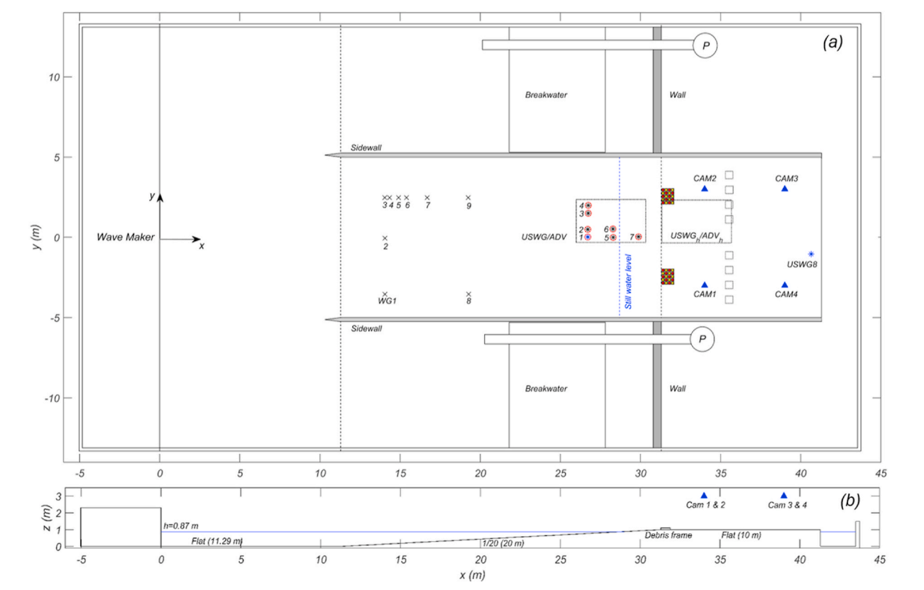
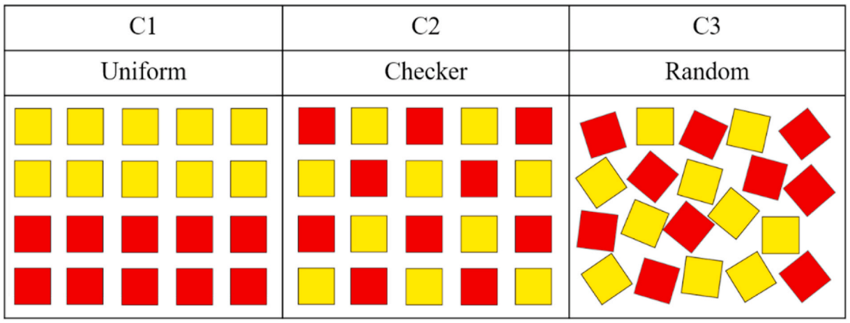
This example examines tsunami-driven debris spreading on a flat, frictional testbed and compares HydroUQ + MPM simulations to the laboratory findings of Park et al. (2021) [Park2021]. In the experiments, debris elements of two densities (HDPE plastic and wooden material) were released in groups with varied starting orientations, then driven by a piston-generated solitary wave across a dry, frictional bed toward two square obstacles. Optical measurements tracked final dislocations, local debris velocities, and collision events, alongside the background flow velocity.
We build a matching digital flume in HydroUQ and use the Material Point Method (MPM) (ClaymoreUW, multi-GPU [Bonus2025ClaymoreUW]) to:
Reproduce the wave forcing (tsunami-like wave) and bed friction conditions in the OSU DWB flume.
Initialize debris groups with HPDE plastic-like properties in arrayed orientations.
Record wave gauge elevations, debris motion, and fluid-debris loads on obstacles.
While this example restricts itself to a subset of behaviors explored in Park et al. 2021, a motivated user could assemble a simulation campaign which targets the following behaviors for comparison:
Asymmetric pair interaction: observe if higher-density debris influences the mean longitudinal displacement of the lighter mate, whereas the lighter element exerts negligible influence on the heavier one.
Orientation insensitivity: verify whether initial group orientation shows any measurable effect on final displacement.
Obstacle effects: check if obstacle rows alter passage and collision probability; if lighter debris tends toward more collisions than heavier debris—except in mixed groups, where lighter debris might show reduced collision probability.
Field context: examine if the reflected wave and debris-debris interactions modulate spreading and collision statistics, and whether element density remains the dominant predictor of collision risk.
4.7.2. Set-Up
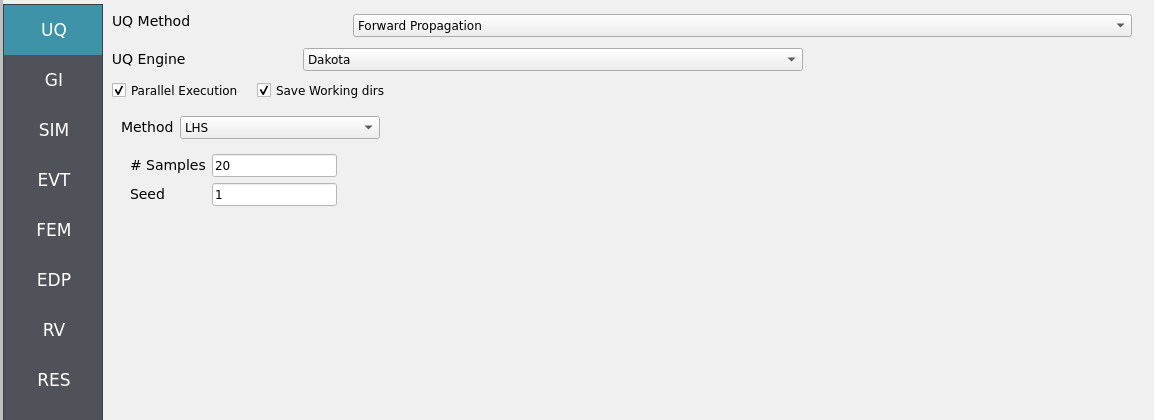
4.7.2.1. Step 1: UQ
Configure Forward sampling to explore structural/material uncertainty under a fixed hydrodynamic signal.
Engine: Dakota
Forward Propagation: Sampling method (e.g., LHS) with
samples(e.g.,20) and a reproducibleseed(e.g.,1).
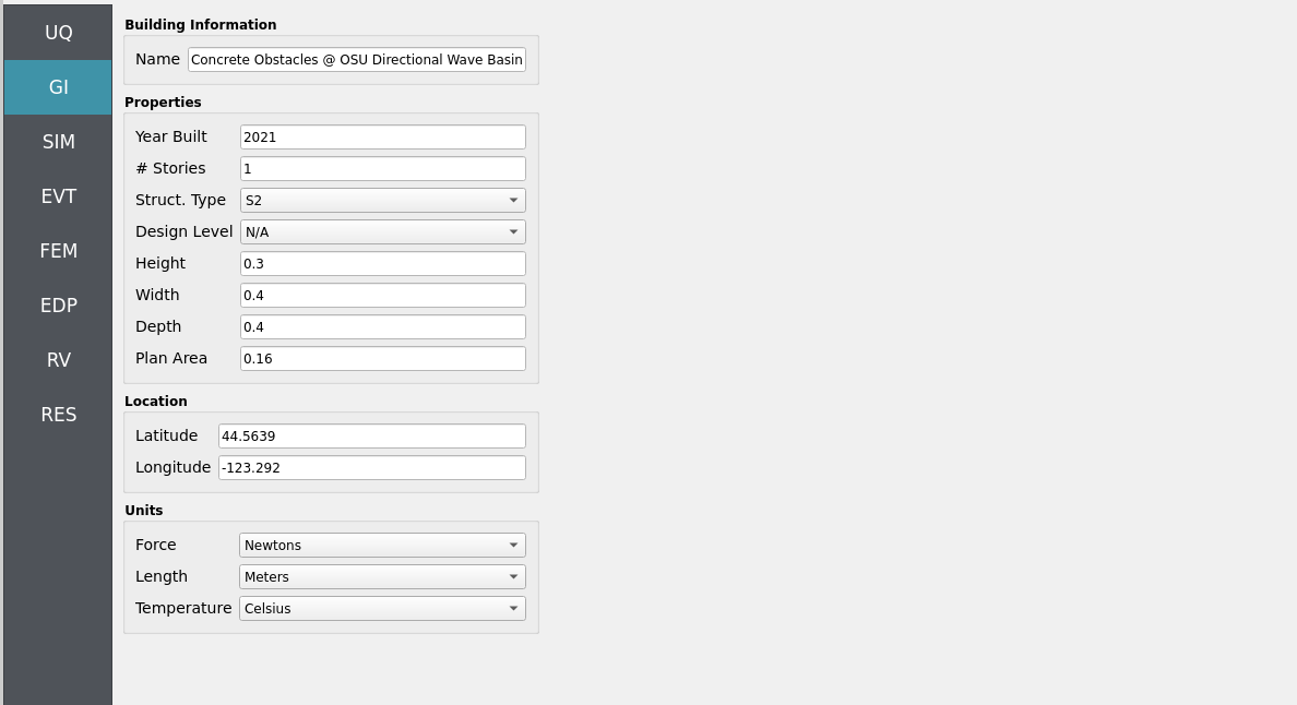
4.7.2.2. Step 2: GI
Set General Information and Units consistent with experiments (length, time, density, gravity). Record project metadata.
Structure name:
Concrete Obstacles @ OSU Directional Wave BasinUnits: choose a consistent set (e.g., N-m-s or kips-in-s)
Note
Keep GI, SIM, EVT, and FEM units consistent. Match MPM’s length/time scales and OpenSees integration settings (e.g., time step). Verify any force/unit conversions used during load mapping.
4.7.2.3. Step 3: SIM
The structural model is as follows: a single-story Multi-Degree-of-Freedom system (MDOF, see Multiple Degrees of Freedom (MDOF)) replicating a structural box in the experimental tests.
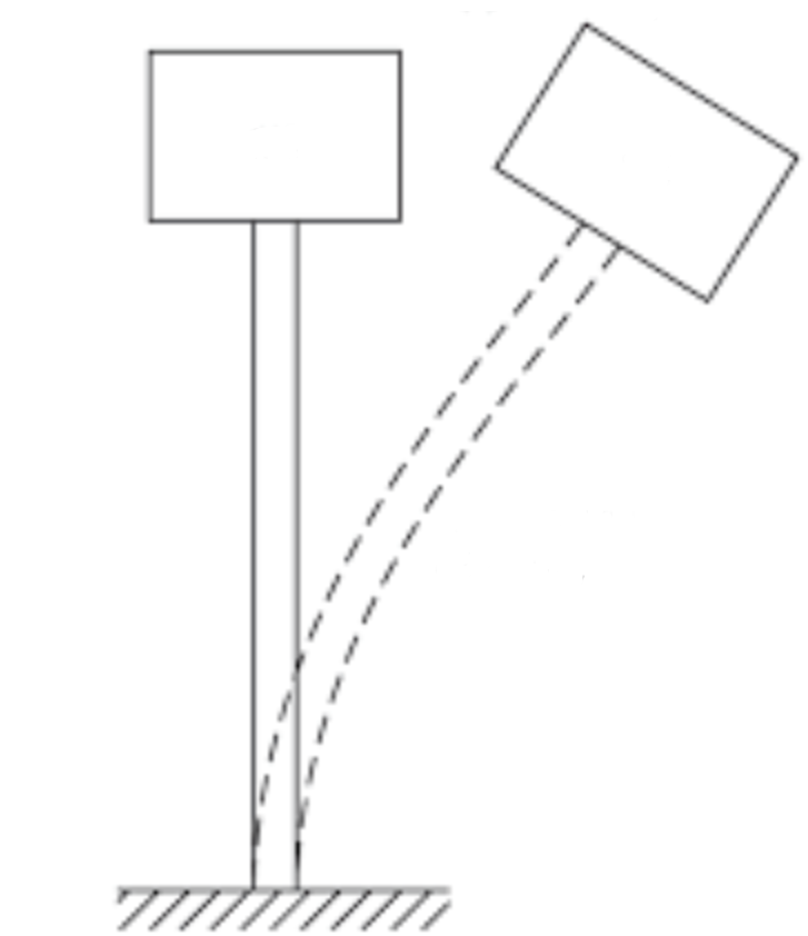
Fig. 4.7.2.3.1 Schematic of a single-story MDOF structure representing a structural box undergoing deflection from MPM derived hydrodynamic loading.
Note
The structure will be represented initially as a rigid boundary in MPM to recover local hydrodynamic forces at grid nodes for direct comparison with load-cell data. Structural dynamic response is added later by mapping these loads onto an OpenSees model defined here in the SIM panel with analysis options set in the FEM panel.
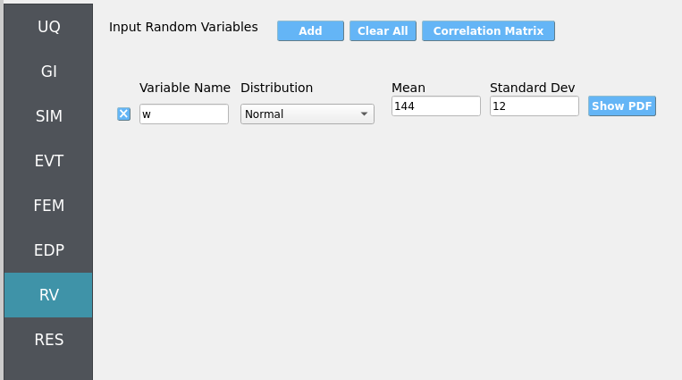
Uncertain structural properties (treated as RVs; see Step 7):
w: Weight. Mean144, stdev12
Bind parameters via setting alphabetic characters in the variable input boxes (e.g., w) so the RV panel recognizes and manages them automatically.
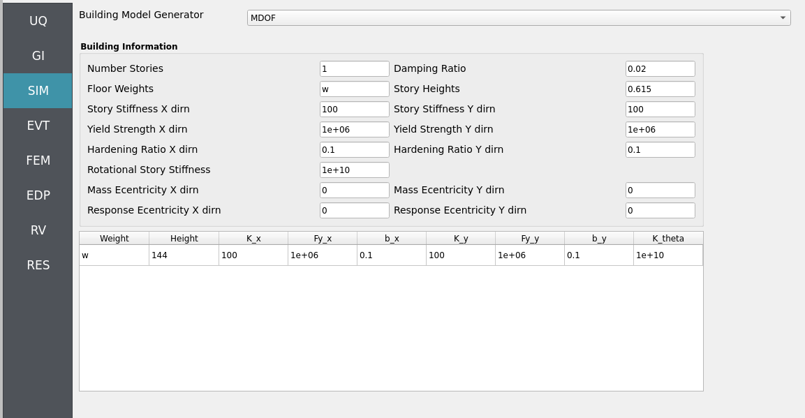
While not necessary to have, we show the template OpenSees model for your reference. The script generated in the backend by the MDOF module resembles the following, MDOF.tcl:
Click to expand the OpenSees input file used for this example
 1model BasicBuilder -ndm 3 -ndf 6
 2pset w 144.0
 3node 2 0 0 576 -mass $w $w  0.0  0.0  0.0  0.0
 4fix 2 0 0 1 1 1 0
 5node 1 0 0 0
 6fix 1 1 1 1 1 1 1
 7uniaxialMaterial Steel01 1 1e+06 100 0.1
 8uniaxialMaterial Steel01 2 1e+06 100 0.1
 9uniaxialMaterial Elastic 3 1e+10
10element zeroLength 1 1 2 -mat 1 2 3 -dir 1 2 6 -doRayleigh
4.7.2.4. Step 4: EVT
In this walk-through we will give a detailed step-by-step configuration of the MPM EVT module.
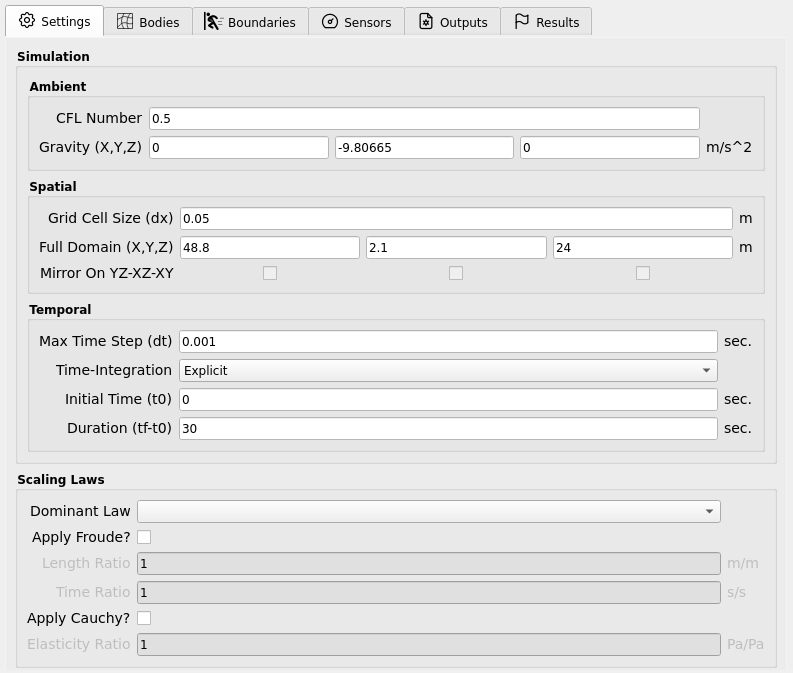
Settings
Open Settings. Here we set the simulation time, the time step, and the grid resolution, among other pre-simulation decisions.
Bodies
Geometry
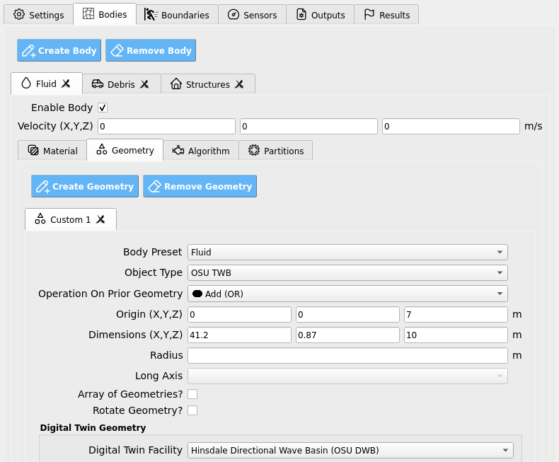
Fluid geometry
Open Bodies / Fluid / Geometry. Here we set the geometry of the flume’s fluid. Note that it is simply a rectangular prism which will be automatically modified to be flush with the defined bathymetry coordinates.
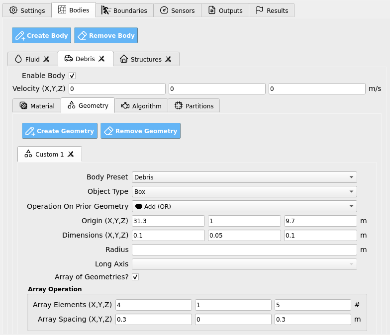
Debris geometry:
Open Bodies / Debris / Geometry. Here we set the debris properties, such as the number of debris, the size of the debris, and the spacing between the debris. Rotation is another option, though not used in this example. We’ve elected to use an 4 x 5 grid of debris (longitudinal axis parallel to long-axis of the flume).
Material
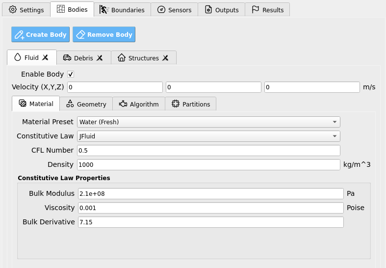
Fluid material:
Open Bodies / Fluid / Material. Here we set the material properties of the fluid. You may choose to use a realistic bulk modulus value of 2.1 GPa for the water, or you may soften it to 0.21 GPa to accelerate the simulation and reduce numerical stiffness with fairly minimal changes in our final results.
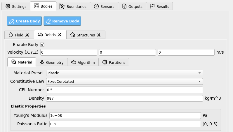
Debris material:
Moving onto the creation of an ordered debris array, we set the debris properties in the Bodies / Debris / Material tab. We will assume debris are made of HDPE plastic, as in experiments by Park et al. 2021 [Park2021], Mascarenas 2022 [Mascarenas2022], and Shekhar et al. 2020 [Shekhar2020], and set properties accordingly. Motivated readers are encouraged to try to replicate the wooden debris from Park et al. 2021 as well. Note that both the wooden and HDPE debris were given HDPE base-plates so that friction coefficients against the flume floor remained constant.
Algorithm
Open Bodies / Fluid / Algorithm. Here we set the algorithm parameters for the simulation. This is an advanced feature of the MPM module, it is best not to alter it too much. We choose to apply F-Bar antilocking to aid in the pressure field’s accuracy on the fluid. The associated toggle must be checked, and the antilocking ratio set to 0.9, loosely. For full bulk modulus water, you may need to increase this value to alleviate numerical stiffness.
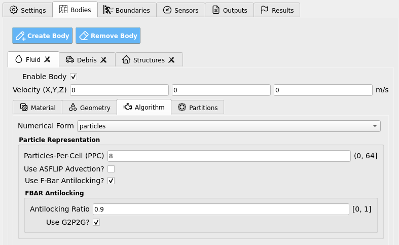
In Bodies / Debris / Algorithm we set debris for compatibility with the fluid as follows: ASFLIP is turned on and F-Bar antilocking is turned off. We keep ASFLIP tuning values at their default of zero as we do not need advanced behavior in this example.

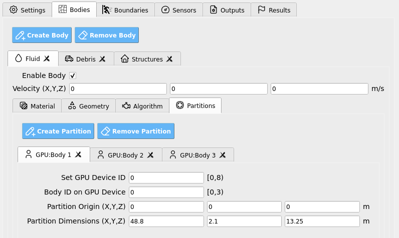
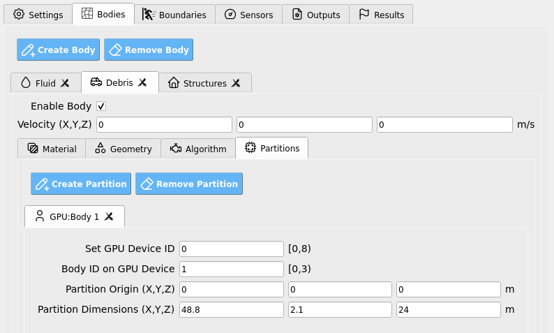
Partitions:
Open Bodies / Fluid / Partitions. This is an advanced feature of the MPM module which allows us to partition material bodies across hardware devices to optimize simulations. These may be kept as their default values, which have already been set for compatibility on the remote HPC system.
Next, Bodies / Debris / Partitions defines a partition where the debris may exist in our flume domain and defines the hardware device (i.e., GPU) that they will be simulated on. Keep this as the default unless you are an advanced user.
Structure:
Finally, open Bodies / Structures. Uncheck the box that enables this body. We will not model the structure as a deformable MPM material body in this example, instead, we will approximate it as a rigid MPM boundary a few steps from now. After the MPM simulation we will map loads from the boundary to an OpenSees structure for structural analysis, see Steps 3 and 5 for configuration.
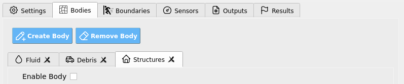
Fig. 4.7.2.4.1 HydroUQ Bodies Structures GUI
Boundaries
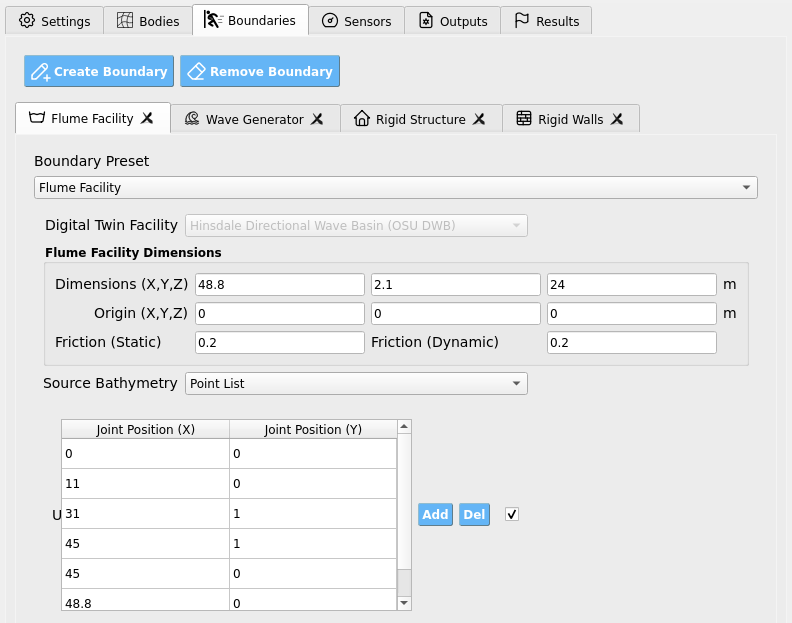
Wave Flume boundary:
Open Boundaries / Flume Facility. We will set the flume boundary to be a rigid body, with a fixed separable velocity condition. Bathymetry joint points should be identical to the ones used in Bodies / Fluid / Geometry. Note that we set static and dynamic friction coefficients to be 0.66. This is approximately as seen in the experiments, but neglects finer-aspects of wetted vs non-wetted contact, etc.
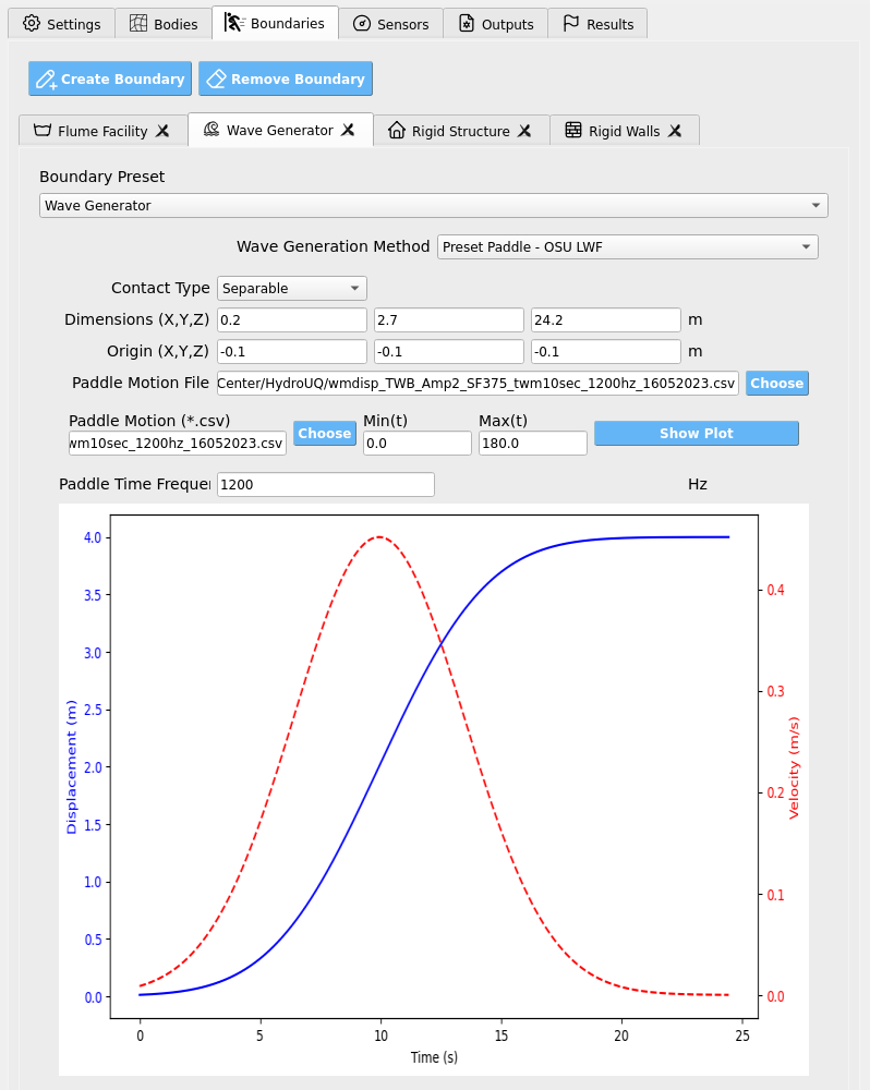
Wave Generator:
Open Boundaries / Wave Generator. Fill in the appropriate file-path for the wave generator paddle motion, wmdisp_TWB_Amp2_SF375_twm10sec_1200hz_16052023.csv. It is designed to produce tsunami-like waves after broaching the bathymetry crest.
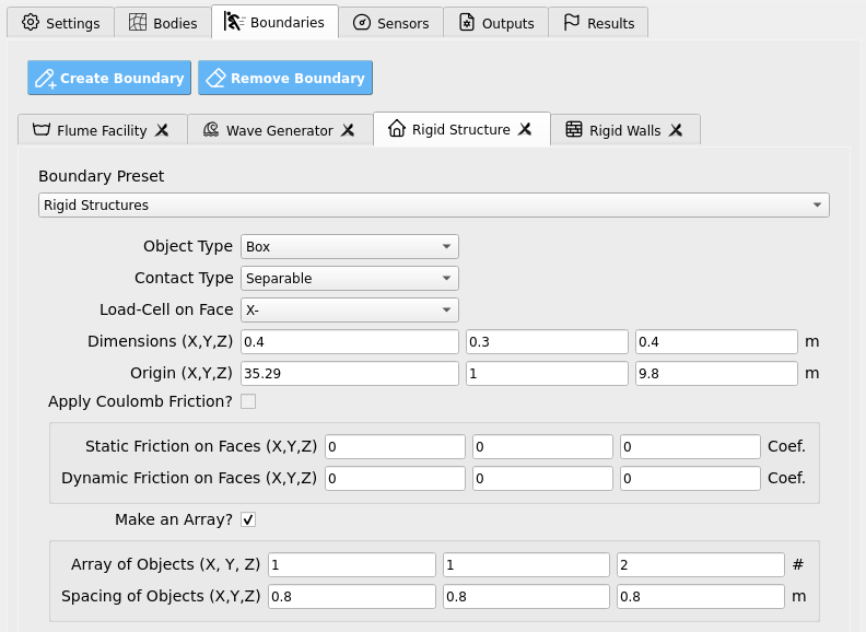
Rigid Structure:
Open Boundaries / Rigid Structure. This is where we will specify the structure as a boundary condition. By doing so, we can determine the exact loads on the rigid boundary grid-nodes, which automatically map to the model defined in the SIM and FEM tab in Steps 3 and 5 for potentially nonlinear UQ structural response analysis.
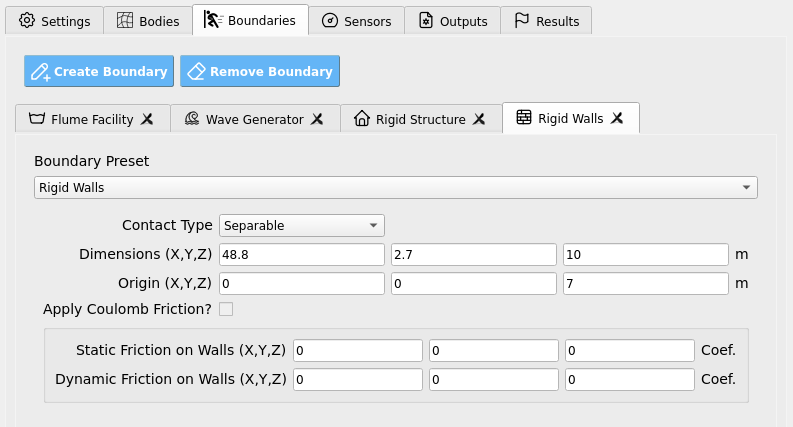
Rigid Walls:
Open Boundaries / Rigid Walls. Set to encompass the flume domain.
Sensors
Wave Gauges:
Open Sensors / Wave Gauges. Set the Use these sensor? box to True so that the simulation will output results for the instruments we set on this page.
Four wave gauges will be defined. The first is located prior to the bathymetry ramp, the second at the foot of the ramp, the third near the bathymetry crest, and the fourth near the debris and structures.
Set the origins and dimensions of each wave gauge to encompass at least one grid-cell in each direction as in the table below. To match experimental conditions, we also apply a 30 Hz sampling rate to the wave gauges.
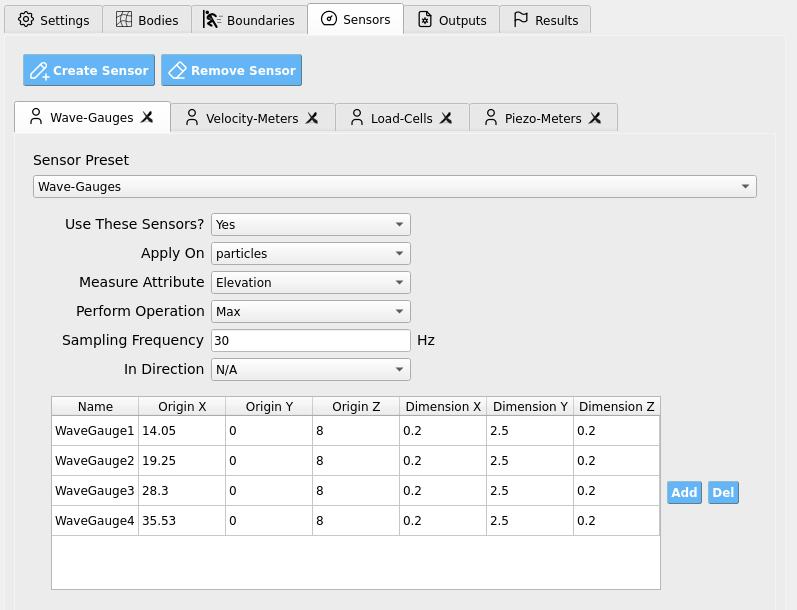
These wave gauges will read all numerical bodies (i.e. particles) within their defined regions at every sampling step and will report the highest elevation value (Position Y) of a contained body as the free-surface elevation at that gauge. The results are written into our sensor results files which we will later analyze.
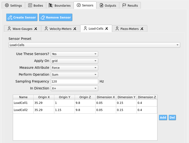
Load Cells:
Open Sensors / Load Cells. Set the Use these sensor? box to True so that the simulation will output results for the instruments we set on this page. Two load cells are defined so that we may map loads onto two nodes of our OpenSees structural model which we defined in Steps 3 and 5. Output frequency is set to 120 Hz to capture primary load phenomena. Note that the experiments themselves were not concerned with measuring structural load, as we do here.
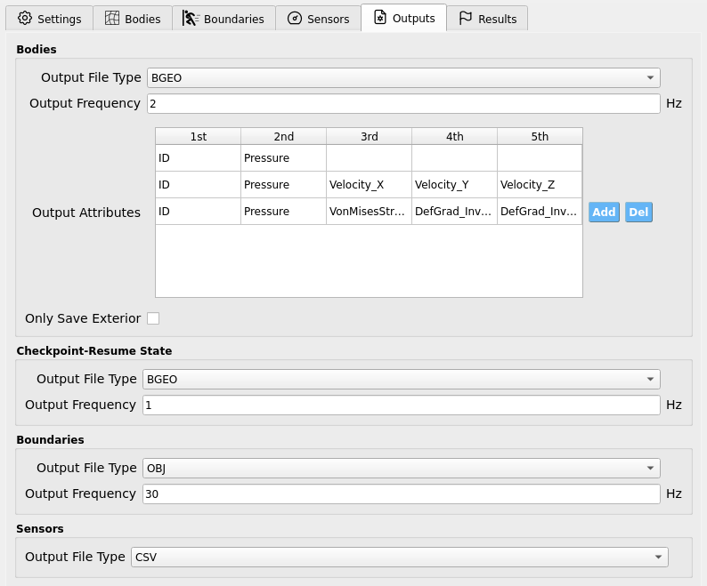
Outputs
Open Outputs. Here we set the non-physical output parameters for the simulation, e.g. attributes to save per frame and file extension types. The particle bodies’ output frequency is set to 2 Hz, meaning the simulation will output results every 0.5 seconds. This is to save disk space and reduce I/O load, but it may be increased if you wish to make animations (e.g., 10 - 30 Hz). Fill the rest of the data in the figure into your GUI to ensure all your outputs match this example. You may alter output attributes if you are an advanced user familiar with ClaymoreUW attributes and wish to perform more advanced analysis.
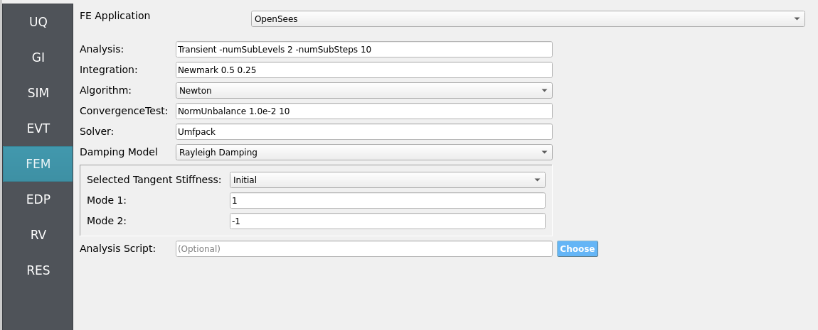
4.7.2.5. Step 5: FEM
This example insofar focused on hydrodynamic forces measured on rigid structures. To perform true structural response analysis, map recovered boundary loads to an OpenSees model in SIM and configure dynamic analysis here as in other HydroUQ tutorials.
Solver: OpenSees dynamic analysis. Check:
Integration step compatible with MPM sensor output interval.
Algorithm/convergence tolerances suitable for expected nonlinearity.
Damping model as needed (e.g., Rayleigh).
4.7.2.6. Step 6: EDP
Select Engineering Demand Parameters (EDPs) to summarize response:
Peak Floor Acceleration (PFA)
Root Mean Square Acceleration (RMSA)
Peak Floor Displacement (PFD)
Peak Interstory Drift (PID)
Note that other quantities of interest (QoI) are theoretically obtainable from HydroUQ, if the custom EDP module is configured. E.g.:
Wave: free-surface elevation η(t) at gauges.
Debris motion: longitudinal displacement (forward/back), lateral spreading angle, stack interaction metrics (contact counts/overturns).
Loads: obstacle force time histories (impact peaks, impulses).
4.7.2.7. Step 7: RV
Define distributions for structural RV:
Structural
w: Normal (mean144, stdev12)
For future UQ, consider:
Debris: mass variance, friction coefficients (debris-apron, debris-debris).
Wave: amplitude/period tolerance relative to piston motion.
Obstacles: small misalignment/placement tolerance.
4.7.3. Simulation
This case was executed on TACC Stampede3 using 2x NVIDIA H100 GPUs on a single node (queue: h100).
Simulated physical time: 30 seconds. Wall time: 180 minutes (allow ample Max Run Time in job settings).
Important
Provide generous Max Run Time, on the order of 180 minutes, to complete the run and post-processing before scheduler limits are reached.
Warning
Keep sensor regions, counts, sampling rates, and output frequencies reasonable—excess I/O can dominate runtime.
Outputs
Sensor CSVs (gauges, debris CoM, loads) at your chosen rates.
Particle/field snapshots (e.g., BGEO/VTK) for visualization/diagnostics.
4.7.4. Analysis
Accessing Results and Simulation Files
When the simulation job has been completed, the results and simulation files will be available on the remote system for retrieval or remote post-processing.
Retrieving the results.zip, templatedir.zip, workdir.tar.gz, and MPM folders will allow you to analyze all of the simulation output (e.g., hydrodynamic, structural, uncertainty quantification).
results.zip: Contains primary uncertainty quantification output and MPM sensor files. This will be the primary place for analysis.templatedir.zip: Contains template and workflow files for the job. This is an important resource for debugging your workflows.workdir.tar.gz: Contains the working directories in which each unique simulation was ran. This is where structural response uncertainty is expanded on typically.MPM: Contains all the MPM simulation files. Includes the raw particle output frames which can be used to create animations or to perform more advanced post-processing.
The most straightforward way to retrieve the most important files, results.zip and templatedir.zip, is by clicking the GET From DesignSafe button in HydroUQ.

Fig. 4.7.4.1 HydroUQ GET From DesignSafe button, which opens up a jobs table of all your remote simulations.
Then, right-click on your job (if it is finished) and select Retrieve Data. This will download results.zip and templatedir.zip.
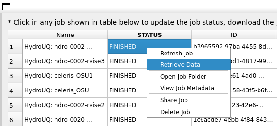
Fig. 4.7.4.2 Locating the Retrieve Data button in the HydroUQ remote jobs table.
HydroUQ will then automatically unzip them into results and templatedir, which will be located in {your_path}/HydroUQ/RemoteWorkDir/tmp.SimCenter. On most systems, this will be ~/Documents/HydroUQ/RemoteWorkDir/tmp.SimCenter, but you can check by clicking on Files / Preferences on the upper-left corner of HydroUQ.
To retrieve workdir.tar.gz and MPM, there are two approaches:
You can right-click on your job within HydroUQ and select
Open Job Folderto be taken directly to the Design Safe web-page displaying all remote files.
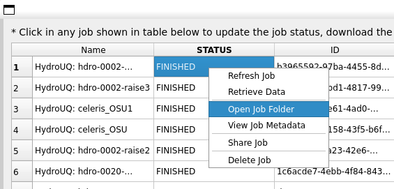
Fig. 4.7.4.3 Locating the Open Job Folder button in the HydroUQ remote jobs table.
You can manually navigate to the designsafe-ci.org website. For the latter, login and go to
Upper-right Drop-down/Job Status.

Fig. 4.7.4.4 Locating the job files on DesignSafe
Check if the job has finished in the central vertical drawer by refreshing the page. If it has, click View Details.
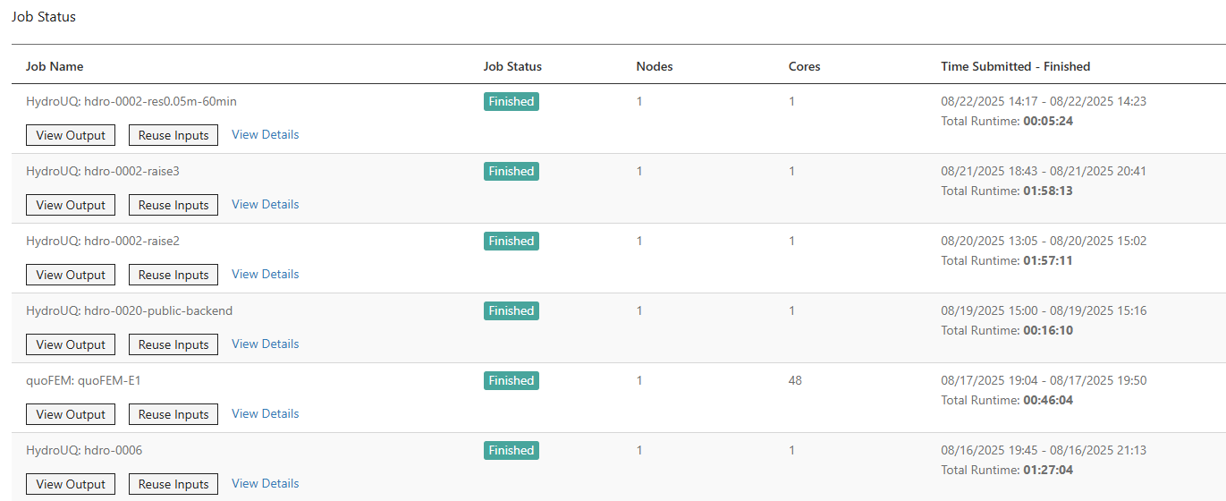
Fig. 4.7.4.5 Job status is finished on DesignSafe
Once the job is finished, the output files should be available in the directory which the analysis results were sent to
Find the files by clicking View Output.
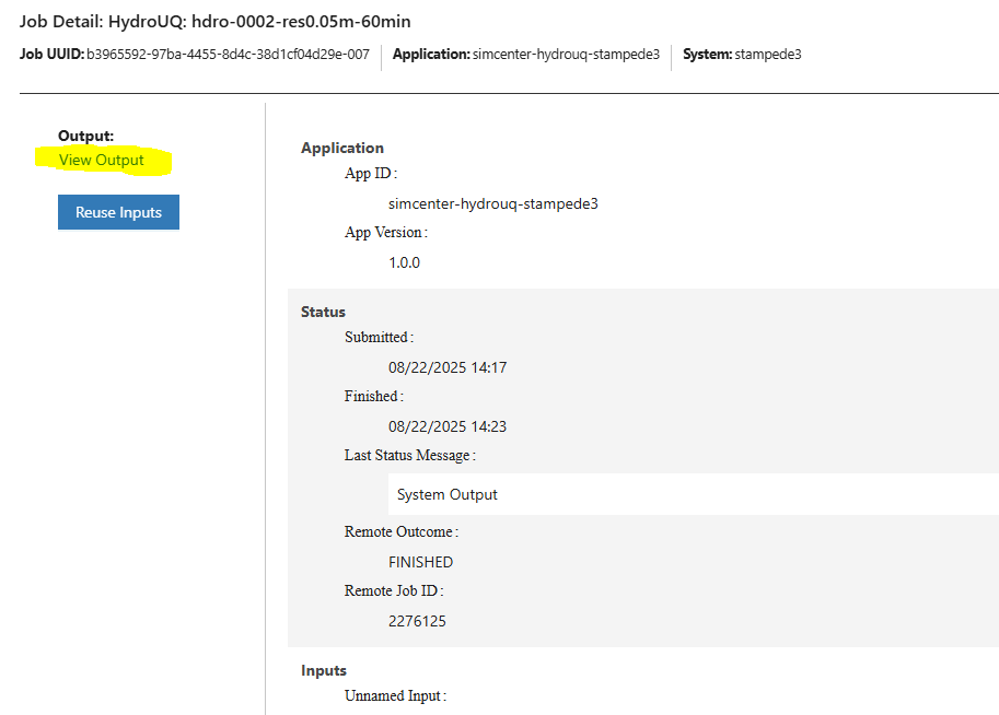
Fig. 4.7.4.6 Viewing the job files on DesignSafe
After navigating to your job folder by one of two ways, it is time to move files for processing. Move important files to somewhere in My Data/ for easier processing. Use the extractor tool available on DesignSafe to unzip the results.zip, workdir.tar.gz, and templatedir.zip folders natively on DesignSafe.
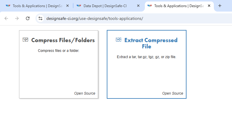
Fig. 4.7.4.7 Extracting the results.zip folder on DesignSafe
Alternatively, you may directly download the zipped folders to your PC, which will require you to use the DesignSafe zip tool on the MPM folder prior.
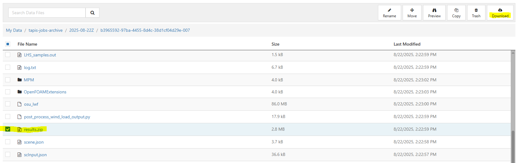
Fig. 4.7.4.8 Download button on DesignSafe shown in red
Locate the downloaded zip folders and extract them somewhere convenient. The HydroUQ local or remote work directory on your computer is a good option.
Warning
Files in the HydroUQ local and remote working directories may be erased if another simulation is set up in HydroUQ, so keep a backup if you wish to maintain the files.
Particle geometry files often have a BGEO extension and are located in the MPM folder. Open with Side FX Houdini Apprentice (free to use) to look at MPM results in high-detail, or use the PartIO library.
HydroUQ’s sensor/probe/instrument output is available in {your_path}/HydroUQ/RemoteWorkDir/tmp.SimCenter/results/ as CSV files. You may process these files as you wish, most opt to use custom Python scripts or Excel due to their simplicity.
Note
For convenience, HydroUQ also includes basic plotting of all sensors files in the EVT / Results tab. Click Post-Process Sensors, configure the drop-down boxes for the sensor you wish to view, and then click Plot.
Plotting the wave gauges shows the development of a tsunami-like wave as it propagates from the piston wave maker and over the harbor bathymetry.
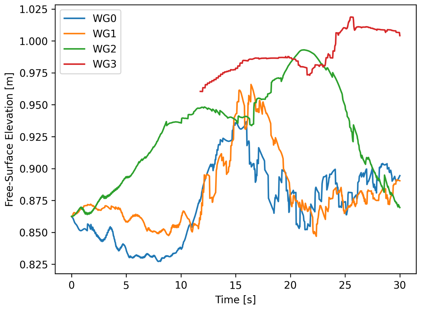
Fig. 4.7.4.9 Simulated free-surface elevations at the wave gauges in MPM.
Compared against experiments we see, as in [Bonus2023Dissertation], the following free-surface signals:
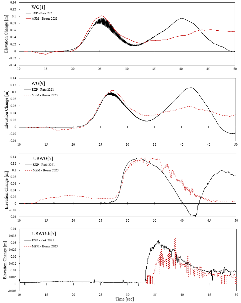
Fig. 4.7.4.10 Simulated free-surface elevations at the wave gauges in MPM from Bonus 2023 against Park et al. 2021.
Load-cell data shows an initially high peak force from debris impact, followed by some damming forces and eventually just hydrodynamic drag.
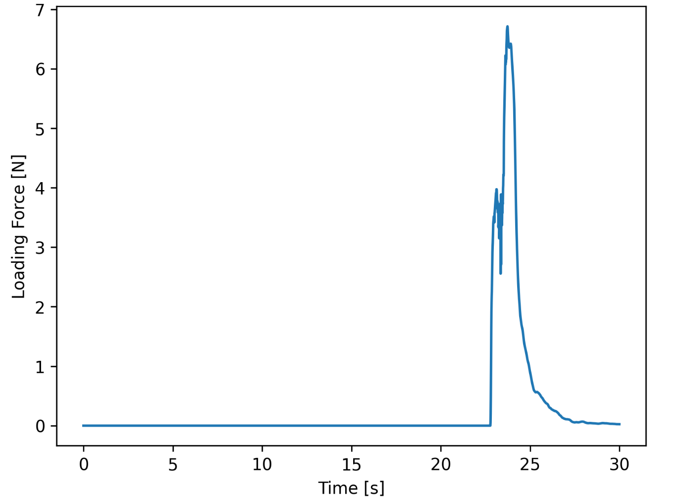
Fig. 4.7.4.11 Simulated load-cell forces in MPM. These are later mapped onto an OpenSees structure for dynamic response analysis.
Structural Analysis
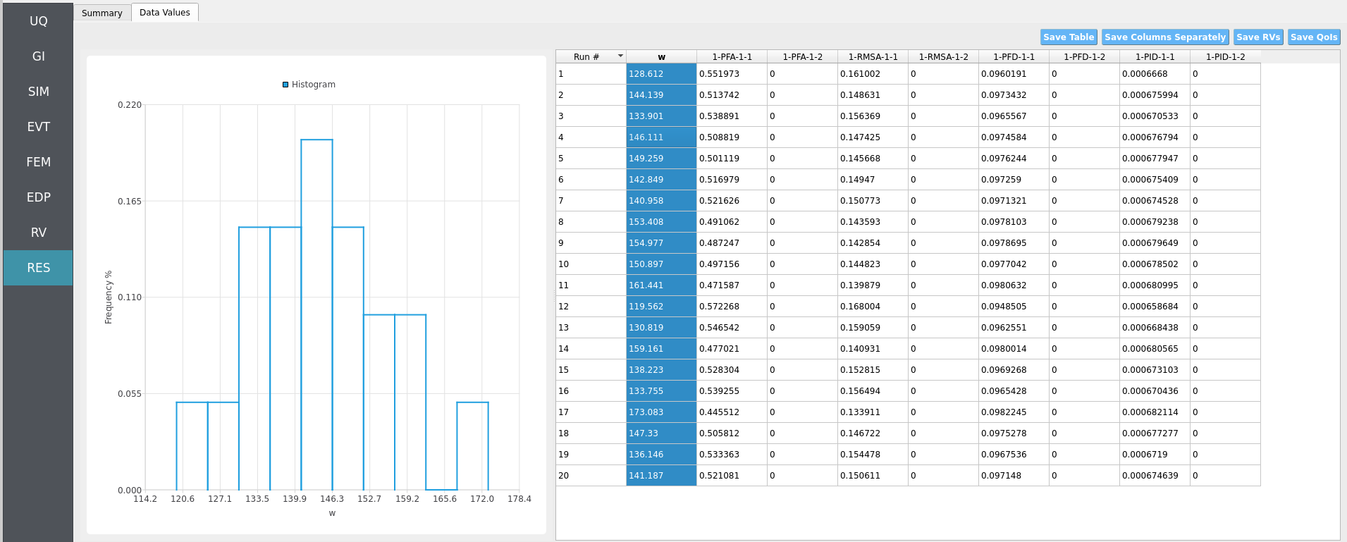
Returning to our primary HydroUQ workflow, which concerns uncertainty in structural response, we may now view the final results in the RES tab. Clicking Summary on the top-bar, a statistical summary of results is shown below:
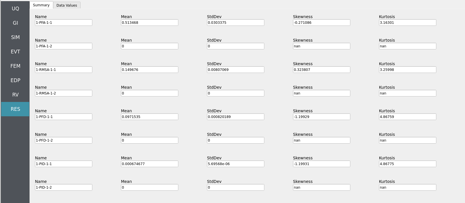
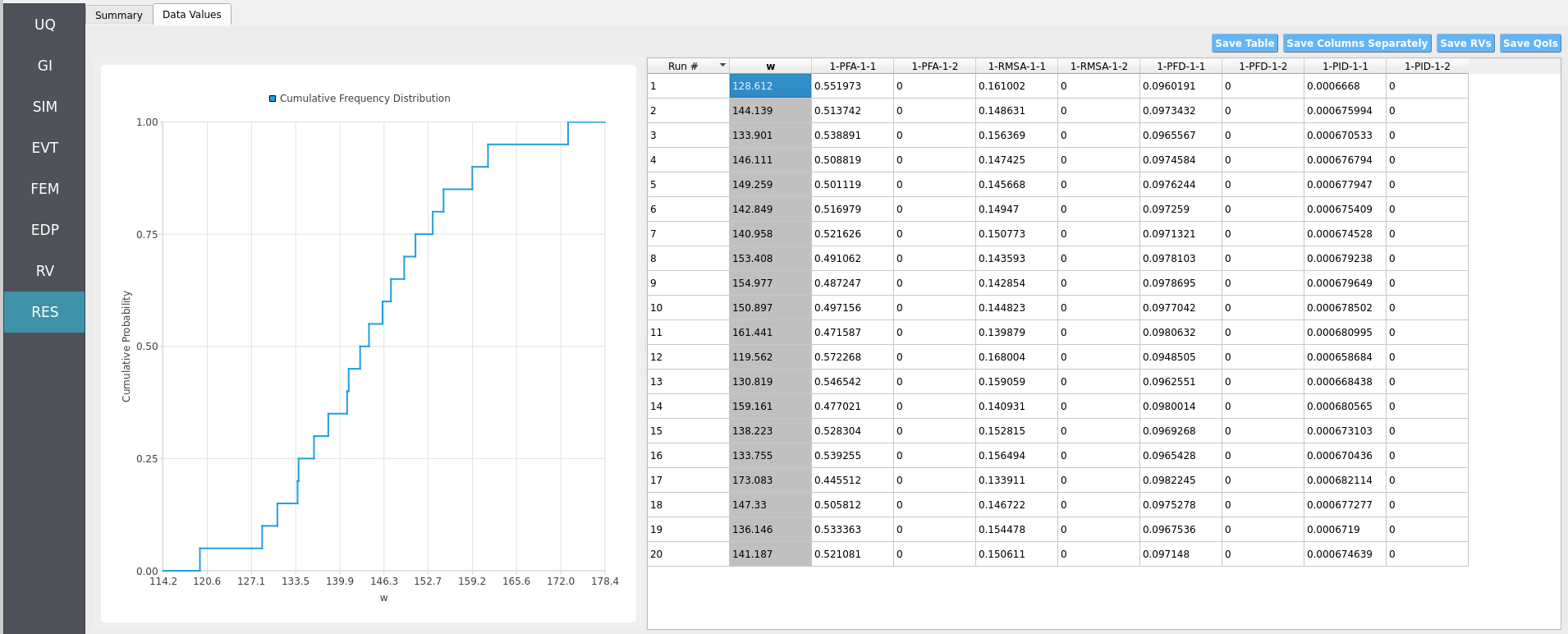
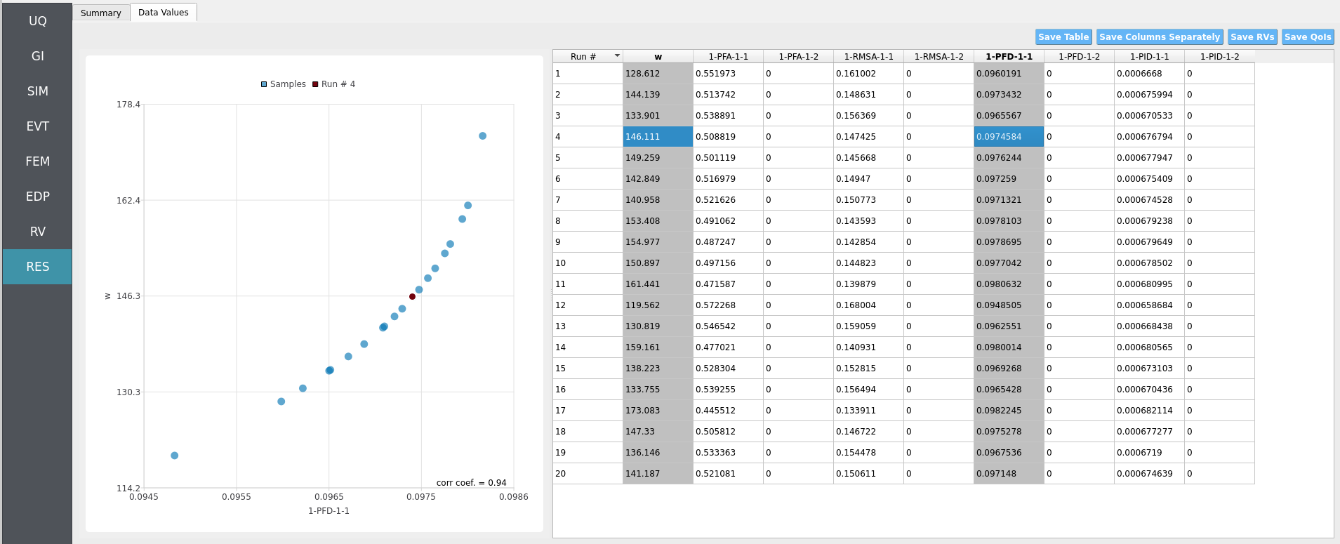
Clicking Data Values on the top-bar shows detailed histograms, cumulative distribution functions, and scatter plots relating the dependent and independent variables:
Note
In the Data Values tab, left- and right-click column headers to change plot axes; selecting a single column with both clicks displays frequency and CDF plots.
Note
Use consistent Froude similitude scaling when comparing numerical simulations, experiments, and full-scale scenarios. For cross-method comparisons, adopt identical debris footprints, friction models, probe placement, and other pertinent parameters to reduce bias.
For more advanced analysis, export results as a CSV file by clicking Save Table on the upper-right of the application window. This will save the independent and dependent variable data. I.e., the Random Variables you defined and the Engineering Demand Parameters determined from the structural response per each simulation.
To save your simulation configuration with results included, click File / Save As and specify a location for the HydroUQ JSON input file to be recorded to. You may then reload the file at a later time by clicking File / Open. You may also send it to others by email or place it in an online repository for research reproducibility. This example’s input file is viewable at Reproducibility.
To directly share your simulation job and results in HydroUQ with other DesignSafe users, click GET from DesignSafe. Then, navigate to the row with your job and right-click it. Select Share Job. You may then enter the DesignSafe username or usernames (comma-separated) to share with.
Important
Sharing a job requires that the job was initially ran with an Archive System ID (listed in the GET from DesignSafe table’s columns) that is not designsafe.storage.default. Any other Archive System ID allows for sharing with DesignSafe members on the associated project. See Jobs for more details.
4.7.5. Conclusions
HydroUQ’s MPM implementation reproduced the incoming wave signal and qualitative trends in debris motion on a frictional bed reported by Park et al. (2021) for the subset case examined, which was concerned with HDPE plastic debris in an array orientation mobilizing into two fixed structural boxes by a tsunami-like wave.
As a next step, motivated readers may seek to reproduce other findings from Park et al. (2021), including:
Density-driven asymmetry: does the heavier element in a pair bias the longitudinal displacement of the lighter one, while the reverse influence was negligible?
Initial orientation of debris groups: do they show no meaningful effect on final dislocation in runs, or is there an underlying trend not seen in experiments due to the limited parameter space?
Obstacle interactions: do baseline cases show higher collision probability for lighter debris; in mixed-density groups, do the lighter debris exhibit a lower collision probability than in single-density runs?
Reflections and interactions: do these phenomena (wave reflection off boundaries and debris-debris contact) modulate local spreading and collisions, or does element density remain the dominant factor governing collision likelihood?
4.7.6. References
Park, H., Koh, M.-J., Cox, D. T., Alam, M. S., & Shin, S. (2021). Experimental study of debris transport driven by a tsunami-like wave: Application for non-uniform density groups and obstacles. Coastal Engineering, 166, 103867. https://doi.org/https://doi.org/10.1016/j.coastaleng.2021.103867
Bonus, Justin (2023). “Evaluation of Fluid-Driven Debris Impacts in a High-Performance Multi-GPU Material Point Method.” PhD thesis. University of Washington, Seattle.
Bonus, J., & Arduino, P. (2025). ClaymoreUW. Zenodo. https://doi.org/10.5281/zenodo.15128706
4.7.7. Reproducibility
Random seed(s):
1(set in UQ)App version: HydroUQ v4.2.0 (or current)
Solver: MPM (ClaymoreUW, multi-GPU)
Hardware: TACC Lonestar6 or Stampede3, 3x A100 or 4x H100 (single node,
gpu-a100orh100queue)Simulated time: 30 seconds; Wall time: 3 hours
Sensor sampling: wave-gauges 120 Hz; particle output 2-10 Hz
Input: The HydroUQ input file is as follows: input.json , is used:
Click to expand the HydroUQ input file used for this example
1{
2 "Applications": {
3 "EDP": {
4 "Application": "StandardEDP",
5 "ApplicationData": {
6 }
7 },
8 "Events": [
9 {
10 "Application": "MPM",
11 "ApplicationData": {
12 },
13 "EventClassification": "Hydro",
14 "defaultMaxRunTime": "1440",
15 "driverFile": "sc_driver",
16 "inputFile": "scInput.json",
17 "maxRunTime": "120",
18 "programFile": "osu_lwf",
19 "publicDirectory": "./"
20 }
21 ],
22 "Modeling": {
23 "Application": "MDOF_BuildingModel",
24 "ApplicationData": {
25 }
26 },
27 "Simulation": {
28 "Application": "OpenSees-Simulation",
29 "ApplicationData": {
30 }
31 },
32 "UQ": {
33 "Application": "Dakota-UQ",
34 "ApplicationData": {
35 }
36 }
37 },
38 "DefaultValues": {
39 "driverFile": "driver",
40 "edpFiles": [
41 "EDP.json"
42 ],
43 "filenameAIM": "AIM.json",
44 "filenameDL": "BIM.json",
45 "filenameEDP": "EDP.json",
46 "filenameEVENT": "EVENT.json",
47 "filenameSAM": "SAM.json",
48 "filenameSIM": "SIM.json",
49 "rvFiles": [
50 "AIM.json",
51 "SAM.json",
52 "EVENT.json",
53 "SIM.json"
54 ],
55 "workflowInput": "scInput.json",
56 "workflowOutput": "EDP.json"
57 },
58 "EDP": {
59 "type": "StandardEDP"
60 },
61 "Events": [
62 {
63 "Application": "MPM",
64 "EventClassification": "Hydro",
65 "example": "OSU DWB",
66 "bodies": [
67 {
68 "algorithm": {
69 "ASFLIP_alpha": 0,
70 "ASFLIP_beta_max": 0,
71 "ASFLIP_beta_min": 0,
72 "FBAR_fused_kernel": true,
73 "FBAR_psi": 0.9,
74 "ppc": 8,
75 "type": "particles",
76 "use_ASFLIP": false,
77 "use_FBAR": true
78 },
79 "geometry": [
80 {
81 "apply_array": false,
82 "apply_rotation": false,
83 "bathymetry": [
84 [
85 0,
86 0
87 ],
88 [
89 11.3,
90 0
91 ],
92 [
93 31.3,
94 1
95 ],
96 [
97 41.3,
98 1
99 ],
100 [
101 41.3,
102 0
103 ],
104 [
105 48.8,
106 0
107 ]
108 ],
109 "body_preset": "Fluid",
110 "facility": "Hinsdale Directional Wave Basin (OSU DWB)",
111 "facility_dimensions": [
112 48.8,
113 2.1,
114 24.0
115 ],
116 "fill_flume_upto_SWL": true,
117 "object": "OSU TWB",
118 "offset": [
119 0,
120 0,
121 7.0
122 ],
123 "operation": "add",
124 "span": [
125 41.2,
126 0.9,
127 10.0
128 ],
129 "standing_water_level": 0.9,
130 "track_particle_id": [
131 "0"
132 ],
133 "use_custom_bathymetry": false,
134 "friction_static": 0.2,
135 "friction_dynamic": 0.2
136 }
137 ],
138 "gpu": 0,
139 "material": {
140 "CFL": 0.5,
141 "bulk_modulus": 210000000,
142 "constitutive": "JFluid",
143 "gamma": 7.15,
144 "material_preset": "Water (Fresh)",
145 "rho": 1000,
146 "viscosity": 0.001
147 },
148 "model": 0,
149 "name": "fluid",
150 "output_attribs": [
151 "ID",
152 "Pressure"
153 ],
154 "partition": [
155 {
156 "gpu": 0,
157 "model": 0,
158 "partition_end": [
159 48.8,
160 2.1,
161 12.0
162 ],
163 "partition_start": [
164 0,
165 0,
166 0
167 ]
168 },
169 {
170 "gpu": 1,
171 "model": 0,
172 "partition_end": [
173 48.8,
174 2.1,
175 24.0
176 ],
177 "partition_start": [
178 0,
179 0,
180 12.0
181 ]
182 },
183 {
184 "gpu": 2,
185 "model": 0,
186 "partition_end": [
187 48.8,
188 2.1,
189 36.0
190 ],
191 "partition_start": [
192 0,
193 0,
194 24.0
195 ]
196 }
197 ],
198 "partition_end": [
199 48.8,
200 2.1,
201 12.0
202 ],
203 "partition_start": [
204 0,
205 0,
206 0
207 ],
208 "target_attribs": [
209 "Position_Y"
210 ],
211 "track_attribs": [
212 "Position_X",
213 "Position_Z",
214 "Pressure"
215 ],
216 "track_particle_id": [
217 0
218 ],
219 "type": "particles",
220 "velocity": [
221 0,
222 0,
223 0
224 ]
225 },
226 {
227 "algorithm": {
228 "ASFLIP_alpha": 0,
229 "ASFLIP_beta_max": 0,
230 "ASFLIP_beta_min": 0,
231 "FBAR_fused_kernel": true,
232 "FBAR_psi": 0,
233 "ppc": 8,
234 "type": "particles",
235 "use_ASFLIP": true,
236 "use_FBAR": false
237 },
238 "geometry": [
239 {
240 "apply_array": true,
241 "apply_rotation": true,
242 "array": [
243 4,
244 1,
245 5
246 ],
247 "body_preset": "Debris",
248 "facility": "Hinsdale Directional Wave Basin (OSU DWB)",
249 "facility_dimensions": [
250 48.8,
251 2.1,
252 24.0
253 ],
254 "fulcrum": [
255 0,
256 0,
257 0
258 ],
259 "object": "Box",
260 "offset": [
261 31.3,
262 1,
263 9.7
264 ],
265 "operation": "add",
266 "rotate": [
267 0,
268 0,
269 0
270 ],
271 "spacing": [
272 0.3,
273 0,
274 0.3
275 ],
276 "span": [
277 0.1,
278 0.05,
279 0.1
280 ],
281 "track_particle_id": [
282 "0"
283 ]
284 }
285 ],
286 "gpu": 0,
287 "material": {
288 "CFL": 0.5,
289 "constitutive": "FixedCorotated",
290 "material_preset": "Plastic",
291 "poisson_ratio": 0.3,
292 "rho": 981,
293 "youngs_modulus": 100000000
294 },
295 "model": 1,
296 "name": "debris",
297 "output_attribs": [
298 "ID",
299 "Pressure",
300 "Velocity_X",
301 "Velocity_Y",
302 "Velocity_Z"
303 ],
304 "partition": [
305 {
306 "gpu": 0,
307 "model": 1,
308 "partition_end": [
309 48.8,
310 2.1,
311 24.0
312 ],
313 "partition_start": [
314 0,
315 0,
316 0
317 ]
318 }
319 ],
320 "partition_end": [
321 48.8,
322 2.1,
323 24.0
324 ],
325 "partition_start": [
326 0,
327 0,
328 0
329 ],
330 "target_attribs": [
331 "Position_Y"
332 ],
333 "track_attribs": [
334 "Position_X",
335 "Position_Z",
336 "Pressure"
337 ],
338 "track_particle_id": [
339 0
340 ],
341 "type": "particles",
342 "velocity": [
343 0,
344 0,
345 0
346 ]
347 },
348 {
349 "algorithm": {
350 "ASFLIP_alpha": 0,
351 "ASFLIP_beta_max": 0,
352 "ASFLIP_beta_min": 0,
353 "FBAR_fused_kernel": true,
354 "FBAR_psi": 0.9,
355 "ppc": 8,
356 "type": "particles",
357 "use_ASFLIP": false,
358 "use_FBAR": true
359 },
360 "geometry": [
361 {
362 "apply_array": false,
363 "apply_rotation": false,
364 "bathymetry": [
365 [
366 0,
367 0
368 ],
369 [
370 11.3,
371 0
372 ],
373 [
374 31.3,
375 1
376 ],
377 [
378 41.3,
379 1
380 ],
381 [
382 41.3,
383 0
384 ],
385 [
386 48.8,
387 0
388 ]
389 ],
390 "body_preset": "Fluid",
391 "facility": "Hinsdale Directional Wave Basin (OSU DWB)",
392 "facility_dimensions": [
393 48.8,
394 2.1,
395 24.0
396 ],
397 "fill_flume_upto_SWL": true,
398 "object": "OSU TWB",
399 "offset": [
400 0,
401 0,
402 7.0
403 ],
404 "operation": "add",
405 "span": [
406 41.2,
407 0.9,
408 10.0
409 ],
410 "standing_water_level": 0.9,
411 "track_particle_id": [
412 "0"
413 ],
414 "use_custom_bathymetry": false
415 }
416 ],
417 "gpu": 1,
418 "material": {
419 "CFL": 0.5,
420 "bulk_modulus": 210000000,
421 "constitutive": "JFluid",
422 "gamma": 7.15,
423 "material_preset": "Water (Fresh)",
424 "rho": 1000,
425 "viscosity": 0.001
426 },
427 "model": 0,
428 "name": "fluid",
429 "output_attribs": [
430 "ID",
431 "Pressure"
432 ],
433 "partition": [
434 {
435 "gpu": 0,
436 "model": 0,
437 "partition_end": [
438 48.8,
439 2.1,
440 12.0
441 ],
442 "partition_start": [
443 0,
444 0,
445 0
446 ]
447 },
448 {
449 "gpu": 1,
450 "model": 0,
451 "partition_end": [
452 48.8,
453 2.1,
454 24.0
455 ],
456 "partition_start": [
457 0,
458 0,
459 12.0
460 ]
461 },
462 {
463 "gpu": 2,
464 "model": 0,
465 "partition_end": [
466 48.8,
467 2.1,
468 36.0
469 ],
470 "partition_start": [
471 0,
472 0,
473 24.0
474 ]
475 }
476 ],
477 "partition_end": [
478 48.8,
479 2.1,
480 24.0
481 ],
482 "partition_start": [
483 48.8,
484 0,
485 12.0
486 ],
487 "target_attribs": [
488 "Position_Y"
489 ],
490 "track_attribs": [
491 "Position_X",
492 "Position_Z",
493 "Pressure"
494 ],
495 "track_particle_id": [
496 0
497 ],
498 "type": "particles",
499 "velocity": [
500 0,
501 0,
502 0
503 ]
504 },
505 {
506 "algorithm": {
507 "ASFLIP_alpha": 0,
508 "ASFLIP_beta_max": 0,
509 "ASFLIP_beta_min": 0,
510 "FBAR_fused_kernel": true,
511 "FBAR_psi": 0.9,
512 "ppc": 8,
513 "type": "particles",
514 "use_ASFLIP": false,
515 "use_FBAR": true
516 },
517 "geometry": [
518 {
519 "apply_array": false,
520 "apply_rotation": false,
521 "bathymetry": [
522 [
523 0,
524 0
525 ],
526 [
527 11.3,
528 0
529 ],
530 [
531 31.3,
532 1
533 ],
534 [
535 41.3,
536 1
537 ],
538 [
539 41.3,
540 0
541 ],
542 [
543 48.8,
544 0
545 ]
546 ],
547 "body_preset": "Fluid",
548 "facility": "Hinsdale Directional Wave Basin (OSU DWB)",
549 "facility_dimensions": [
550 48.8,
551 2.1,
552 24.0
553 ],
554 "fill_flume_upto_SWL": true,
555 "object": "OSU TWB",
556 "offset": [
557 0,
558 0,
559 7.0
560 ],
561 "operation": "add",
562 "span": [
563 41.2,
564 0.9,
565 10.0
566 ],
567 "standing_water_level": 0.9,
568 "track_particle_id": [
569 "0"
570 ],
571 "use_custom_bathymetry": false
572 }
573 ],
574 "gpu": 2,
575 "material": {
576 "CFL": 0.5,
577 "bulk_modulus": 210000000,
578 "constitutive": "JFluid",
579 "gamma": 7.15,
580 "material_preset": "Water (Fresh)",
581 "rho": 1000,
582 "viscosity": 0.001
583 },
584 "model": 0,
585 "name": "fluid",
586 "output_attribs": [
587 "ID",
588 "Pressure"
589 ],
590 "partition": [
591 {
592 "gpu": 0,
593 "model": 0,
594 "partition_end": [
595 48.8,
596 2.1,
597 12.0
598 ],
599 "partition_start": [
600 0,
601 0,
602 0
603 ]
604 },
605 {
606 "gpu": 1,
607 "model": 0,
608 "partition_end": [
609 48.8,
610 2.1,
611 24.0
612 ],
613 "partition_start": [
614 0,
615 0,
616 12.0
617 ]
618 },
619 {
620 "gpu": 2,
621 "model": 0,
622 "partition_end": [
623 48.8,
624 2.1,
625 36.0
626 ],
627 "partition_start": [
628 0,
629 0,
630 24.0
631 ]
632 }
633 ],
634 "partition_end": [
635 48.8,
636 2.1,
637 36.0
638 ],
639 "partition_start": [
640 0,
641 0,
642 24.0
643 ],
644 "target_attribs": [
645 "Position_Y"
646 ],
647 "track_attribs": [
648 "Position_X",
649 "Position_Z",
650 "Pressure"
651 ],
652 "track_particle_id": [
653 0
654 ],
655 "type": "particles",
656 "velocity": [
657 0,
658 0,
659 0
660 ]
661 }
662 ],
663 "boundaries": [
664 {
665 "bathymetry": [
666 [
667 0,
668 0
669 ],
670 [
671 11.3,
672 0
673 ],
674 [
675 31.3,
676 1
677 ],
678 [
679 41.3,
680 1
681 ],
682 [
683 41.3,
684 0
685 ],
686 [
687 48.8,
688 0
689 ]
690 ],
691 "contact": "Separable",
692 "domain_end": [
693 48.8,
694 2.1,
695 24.0
696 ],
697 "domain_start": [
698 0,
699 0,
700 0
701 ],
702 "friction_dynamic": 0.66,
703 "friction_static": 0.66,
704 "object": "Bathymetry",
705 "use_custom_bathymetry": true
706 },
707 {
708 "contact": "Separable",
709 "domain_end": [
710 0.0,
711 2.6,
712 24.1
713 ],
714 "domain_start": [
715 -0.2,
716 -0.1,
717 -0.1
718 ],
719 "file": "..//wmdisp_TWB_Amp2_SF375_twm10sec_1200hz_16052023.csv",
720 "friction_dynamic": 0,
721 "friction_static": 0,
722 "object": "OSU Paddle",
723 "output_frequency": 1200
724 },
725 {
726 "array": [
727 1,
728 1,
729 2
730 ],
731 "contact": "Separable",
732 "domain_end": [
733 35.69,
734 1.3,
735 10.200000000000001
736 ],
737 "domain_start": [
738 35.29,
739 1,
740 9.8
741 ],
742 "friction_dynamic": 0,
743 "friction_static": 0,
744 "object": "Box",
745 "spacing": [
746 0.8,
747 0.8,
748 0.8
749 ]
750 },
751 {
752 "contact": "Separable",
753 "domain_end": [
754 48.8,
755 2.7,
756 17.0
757 ],
758 "domain_start": [
759 0,
760 0,
761 7.0
762 ],
763 "friction_dynamic": 0,
764 "friction_static": 0,
765 "object": "Walls"
766 }
767 ],
768 "computer": {
769 "hpc": "TACC - UT Austin - Lonestar6",
770 "hpc_card_architecture": "Ampere",
771 "hpc_card_brand": "NVIDIA",
772 "hpc_card_compute_capability": 80,
773 "hpc_card_global_memory": 40,
774 "hpc_card_name": "A100",
775 "hpc_queue": "gpu-a100",
776 "models_per_gpu": 3,
777 "num_gpus": 3
778 },
779 "grid-sensors": [
780 {
781 "attribute": "Force",
782 "direction": "X+",
783 "domain_end": [
784 35.339999999999996,
785 1.15,
786 10.200000000000001
787 ],
788 "domain_start": [
789 35.29,
790 1,
791 9.8
792 ],
793 "name": "LoadCell1",
794 "operation": "Sum",
795 "output_frequency": 120,
796 "preset": "Load-Cells",
797 "summary": [
798 [
799 "LoadCell1",
800 35.29,
801 1,
802 9.8,
803 0.05,
804 0.15,
805 0.4
806 ],
807 [
808 "LoadCell2",
809 35.29,
810 1.15,
811 9.8,
812 0.05,
813 0.15,
814 0.4
815 ]
816 ],
817 "toggle": true,
818 "type": "grid"
819 },
820 {
821 "attribute": "Force",
822 "direction": "X+",
823 "domain_end": [
824 35.339999999999996,
825 1.2999999999999998,
826 10.200000000000001
827 ],
828 "domain_start": [
829 35.29,
830 1.15,
831 9.8
832 ],
833 "name": "LoadCell2",
834 "operation": "Sum",
835 "output_frequency": 120,
836 "preset": "Load-Cells",
837 "summary": [
838 [
839 "LoadCell1",
840 35.29,
841 1,
842 9.8,
843 0.05,
844 0.15,
845 0.4
846 ],
847 [
848 "LoadCell2",
849 35.29,
850 1.15,
851 9.8,
852 0.05,
853 0.15,
854 0.4
855 ]
856 ],
857 "toggle": true,
858 "type": "grid"
859 }
860 ],
861 "outputs": {
862 "bodies_output_freq": 2,
863 "bodies_save_suffix": "BGEO",
864 "boundaries_output_freq": 30,
865 "boundaries_save_suffix": "OBJ",
866 "checkpoints_output_freq": 1,
867 "checkpoints_save_suffix": "BGEO",
868 "energies_output_freq": 30,
869 "energies_save_suffix": "CSV",
870 "output_attribs": [
871 [
872 "ID",
873 "Pressure"
874 ],
875 [
876 "ID",
877 "Pressure",
878 "Velocity_X",
879 "Velocity_Y",
880 "Velocity_Z"
881 ],
882 [
883 "ID",
884 "Pressure",
885 "VonMisesStress",
886 "DefGrad_Invariant2",
887 "DefGrad_Invariant3"
888 ]
889 ],
890 "particles_output_exterior_only": false,
891 "sensors_save_suffix": "CSV",
892 "useKineticEnergy": false,
893 "usePotentialEnergy": false,
894 "useStrainEnergy": false
895 },
896 "particle-sensors": [
897 {
898 "attribute": "Elevation",
899 "direction": "N/A",
900 "domain_end": [
901 14.25,
902 2.5,
903 8.2
904 ],
905 "domain_start": [
906 14.05,
907 0,
908 8
909 ],
910 "name": "WaveGauge1",
911 "operation": "Max",
912 "output_frequency": 30,
913 "preset": "Wave-Gauges",
914 "summary": [
915 [
916 "WaveGauge1",
917 14.05,
918 0,
919 8,
920 0.2,
921 2.5,
922 0.2
923 ],
924 [
925 "WaveGauge2",
926 19.25,
927 0,
928 8,
929 0.2,
930 2.5,
931 0.2
932 ],
933 [
934 "WaveGauge3",
935 28.30,
936 0,
937 8,
938 0.2,
939 2.5,
940 0.2
941 ],
942 [
943 "WaveGauge4",
944 35.53,
945 0,
946 8,
947 0.2,
948 2.5,
949 0.2
950 ]
951 ],
952 "toggle": true,
953 "type": "particles"
954 },
955 {
956 "attribute": "Elevation",
957 "direction": "N/A",
958 "domain_end": [
959 19.45,
960 2.5,
961 8.2
962 ],
963 "domain_start": [
964 19.25,
965 0,
966 8
967 ],
968 "name": "WaveGauge2",
969 "operation": "Max",
970 "output_frequency": 30,
971 "preset": "Wave-Gauges",
972 "summary": [
973 [
974 "WaveGauge1",
975 14.05,
976 0,
977 8,
978 0.2,
979 2.5,
980 0.2
981 ],
982 [
983 "WaveGauge2",
984 19.25,
985 0,
986 8,
987 0.2,
988 2.5,
989 0.2
990 ],
991 [
992 "WaveGauge3",
993 28.30,
994 0,
995 8,
996 0.2,
997 2.5,
998 0.2
999 ],
1000 [
1001 "WaveGauge4",
1002 35.53,
1003 0,
1004 8,
1005 0.2,
1006 2.5,
1007 0.2
1008 ]
1009 ],
1010 "toggle": true,
1011 "type": "particles"
1012 },
1013 {
1014 "attribute": "Elevation",
1015 "direction": "N/A",
1016 "domain_end": [
1017 28.5,
1018 2.5,
1019 8.2
1020 ],
1021 "domain_start": [
1022 28.3,
1023 0,
1024 8
1025 ],
1026 "name": "WaveGauge3",
1027 "operation": "Max",
1028 "output_frequency": 30,
1029 "preset": "Wave-Gauges",
1030 "summary": [
1031 [
1032 "WaveGauge1",
1033 14.05,
1034 0,
1035 8,
1036 0.2,
1037 2.5,
1038 0.2
1039 ],
1040 [
1041 "WaveGauge2",
1042 19.25,
1043 0,
1044 8,
1045 0.2,
1046 2.5,
1047 0.2
1048 ],
1049 [
1050 "WaveGauge3",
1051 28.30,
1052 0,
1053 8,
1054 0.2,
1055 2.5,
1056 0.2
1057 ],
1058 [
1059 "WaveGauge4",
1060 35.53,
1061 0,
1062 8,
1063 0.2,
1064 2.5,
1065 0.2
1066 ]
1067 ],
1068 "toggle": true,
1069 "type": "particles"
1070 },
1071 {
1072 "attribute": "Elevation",
1073 "direction": "N/A",
1074 "domain_end": [
1075 35.73,
1076 2.5,
1077 8.2
1078 ],
1079 "domain_start": [
1080 35.53,
1081 0,
1082 8
1083 ],
1084 "name": "WaveGauge4",
1085 "operation": "Max",
1086 "output_frequency": 30,
1087 "preset": "Wave-Gauges",
1088 "summary": [
1089 [
1090 "WaveGauge1",
1091 14.05,
1092 0,
1093 8,
1094 0.2,
1095 2.5,
1096 0.2
1097 ],
1098 [
1099 "WaveGauge2",
1100 19.25,
1101 0,
1102 8,
1103 0.2,
1104 2.5,
1105 0.2
1106 ],
1107 [
1108 "WaveGauge3",
1109 28.30,
1110 0,
1111 8,
1112 0.2,
1113 2.5,
1114 0.2
1115 ],
1116 [
1117 "WaveGauge4",
1118 35.53,
1119 0,
1120 8,
1121 0.2,
1122 2.5,
1123 0.2
1124 ]
1125 ],
1126 "toggle": true,
1127 "type": "particles"
1128 }
1129 ],
1130 "scaling": {
1131 "cauchy_bulk_ratio": 1,
1132 "froude_length_ratio": 1,
1133 "froude_time_ratio": 1,
1134 "use_cauchy_scaling": false,
1135 "use_froude_scaling": false
1136 },
1137 "simulation": {
1138 "cauchy_bulk_ratio": 1,
1139 "cfl": 0.5,
1140 "default_dt": 0.001,
1141 "default_dx": 0.05,
1142 "domain": [
1143 48.8,
1144 2.1,
1145 24.0
1146 ],
1147 "duration": 30.0,
1148 "fps": 2,
1149 "frames": 60,
1150 "froude_scaling": 1,
1151 "froude_time_ratio": 1,
1152 "gravity": [
1153 0,
1154 -9.80665,
1155 0
1156 ],
1157 "initial_time": 0,
1158 "mirror_domain": [
1159 false,
1160 false,
1161 false
1162 ],
1163 "particles_output_exterior_only": false,
1164 "save_suffix": ".bgeo",
1165 "time": 0,
1166 "time_integration": "Explicit",
1167 "use_cauchy_scaling": false,
1168 "use_froude_scaling": false
1169 },
1170 "subtype": "MPM",
1171 "type": "MPM"
1172 }
1173 ],
1174 "GeneralInformation": {
1175 "NumberOfStories": 1,
1176 "PlanArea": 0.16,
1177 "StructureType": "S2",
1178 "YearBuilt": 1990,
1179 "depth": 0.4,
1180 "height": 0.3,
1181 "location": {
1182 "latitude": 44.5639,
1183 "longitude": -123.292
1184 },
1185 "name": "Concrete Obstacles @ OSU's Directional Wave Basin",
1186 "planArea": 0.16,
1187 "stories": 1,
1188 "units": {
1189 "force": "N",
1190 "length": "m",
1191 "temperature": "C",
1192 "time": "sec"
1193 },
1194 "width": 0.4
1195 },
1196 "Modeling": {
1197 "Bx": 0.1,
1198 "By": 0.1,
1199 "Fyx": 1000000,
1200 "Fyy": 1000000,
1201 "Krz": 10000000000,
1202 "Kx": 100,
1203 "Ky": 100,
1204 "ModelData": [
1205 {
1206 "Fyx": 1000000,
1207 "Fyy": 1000000,
1208 "Ktheta": 10000000000,
1209 "bx": 0.1,
1210 "by": 0.1,
1211 "height": 144,
1212 "kx": 100,
1213 "ky": 100,
1214 "weight": "RV.w"
1215 }
1216 ],
1217 "dampingRatio": 0.02,
1218 "height": 0.615,
1219 "massX": 0,
1220 "massY": 0,
1221 "numStories": 1,
1222 "randomVar": [
1223 ],
1224 "responseX": 0,
1225 "responseY": 0,
1226 "type": "MDOF_BuildingModel",
1227 "weight": "RV.w"
1228 },
1229 "Simulation": {
1230 "Application": "OpenSees-Simulation",
1231 "algorithm": "Newton",
1232 "analysis": "Transient -numSubLevels 2 -numSubSteps 10",
1233 "convergenceTest": "NormUnbalance 1.0e-2 10",
1234 "dampingModel": "Rayleigh Damping",
1235 "firstMode": 1,
1236 "integration": "Newmark 0.5 0.25",
1237 "modalRayleighTangentRatio": 0,
1238 "numModesModal": -1,
1239 "rayleighTangent": "Initial",
1240 "secondMode": -1,
1241 "solver": "Umfpack"
1242 },
1243 "UQ": {
1244 "parallelExecution": true,
1245 "samplingMethodData": {
1246 "method": "LHS",
1247 "samples": 20,
1248 "seed": 1
1249 },
1250 "saveWorkDir": true,
1251 "uqType": "Forward Propagation"
1252 },
1253 "correlationMatrix": [
1254 1
1255 ],
1256 "localAppDir": "/home/justinbonus/SimCenter/HydroUQ/build",
1257 "randomVariables": [
1258 {
1259 "distribution": "Normal",
1260 "inputType": "Parameters",
1261 "mean": 144,
1262 "name": "w",
1263 "refCount": 1,
1264 "stdDev": 12,
1265 "value": "RV.w",
1266 "variableClass": "Uncertain"
1267 }
1268 ],
1269 "remoteAppDir": "/home/justinbonus/SimCenter/HydroUQ/build",
1270 "resultType": "SimCenterUQResultsSampling",
1271 "runType": "runningLocal",
1272 "summary": [
1273 ],
1274 "workingDir": "/home/justinbonus/Documents/HydroUQ/LocalWorkDir"
1275}