4.10. Debris-Flow Down a Hill-Slope - Digital Flume (USGS DFF) - MPM
Problem files |
4.10.1. Outline
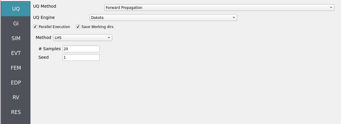
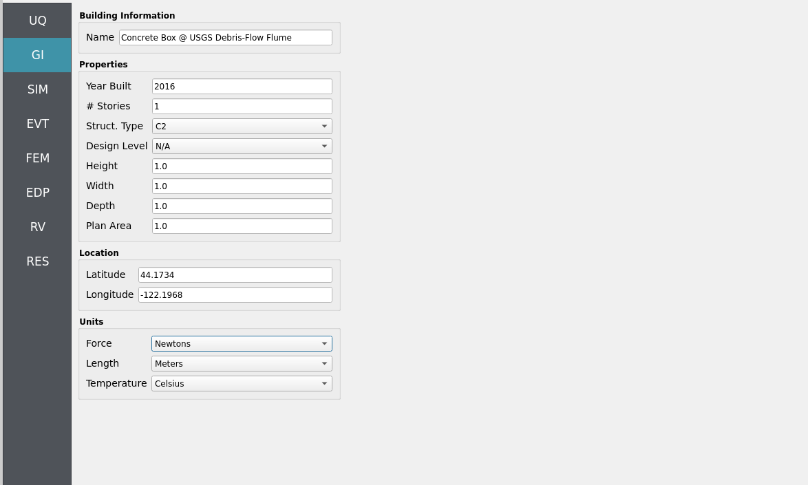
Fig. 4.10.1.1 GUI for the United State Geological Survey’s Debris-Flow Flume (USGS DFF).
This example investigates runup of debris flows ([Iverson2010]) against obstacles by comparing insights from large-scale experiments (e.g., vertical walls vs sloping barriers, [Iverson2016]) at the United State’s Geological Survey’s Debris-Flow Flume (USGS DFF) to a fully 3D Material Point Method (MPM, [Bonus2023Dissertation] and [Bonus2025ClaymoreUW]) simulation in HydroUQ. Guided by the experimental findings (shock-dominated runup at normal walls; pre-shock mass and momentum flux that increases runup on sloping obstacles; runup sensitivity to Froude number and effective basal friction/liquefaction), we construct a dry, high-friction MPM scenario:
A sand mass (Drucker-Prager, dilatant; no pore-pressure coupling) is released on a hillside flume’s crest on a 31 deg slope and accelerates downslope.
At the toe, the flow impacts a raised structural box (an idealized vertical barrier) — the canonical shock-runup regime.
The runout pad is frictional; macro-roughness may be represented either (i) by a Coulomb friction coefficient with a decay layer (computationally light), or (ii) by explicit roughness elements at fine grid spacing (captures grain-scale bouncing and sorting more faithfully).
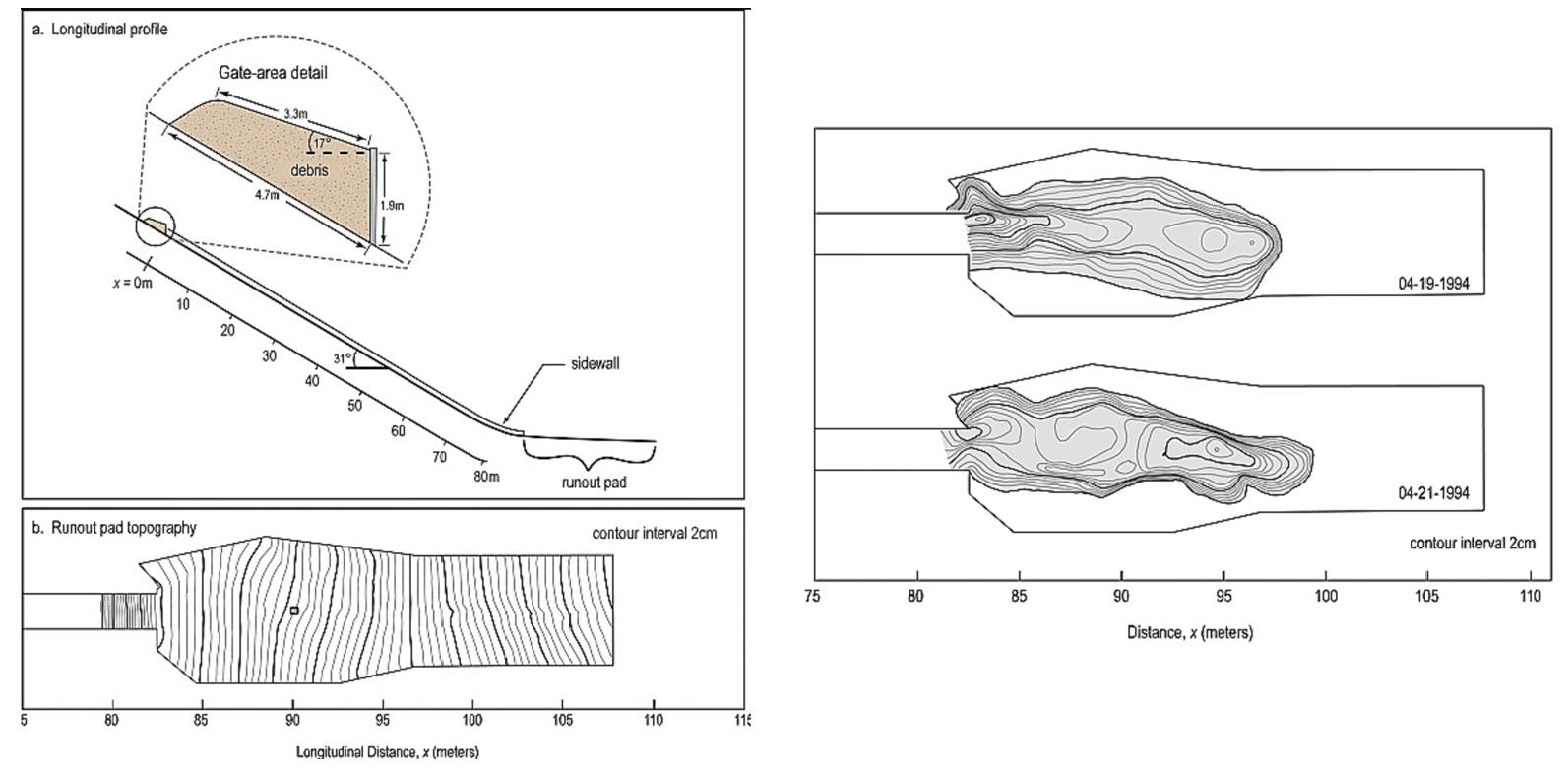
Fig. 4.10.1.2 Schematic of the United State Geological Survey’s Debris-Flow Flume (USGS DFF) in Iverson 2016.
Because our base case is dry (no liquefaction), it represents the upper-friction bound of the experimental phase space: we anticipate strong shock development at the wall, shorter runup than low-friction/liquefied cases, and force histories dominated by a sharp impulse followed by damming. The setup is, however, readily extensible to two-phase MPM or hybrid MPM-CFD to examine the role of pore pressure on runup amplification and predictive skill in “ab initio” vs “data-informed” modes. To connect with the full experimental/analytical picture, we recommend advanced users go beyond this example by tracking and non-dimensionalizing the following quantities of interest (QoIs):
Incoming front Froude number, \(Fr = U_f/\sqrt{g\,h_f}\), with \(U_f\) and \(h_f\) measured at the last up-slope station before impact (pre-shock state).
Runup height at the obstacle, measured as peak free-surface elevation (and center-of-mass rise) along the wall; compare to analytical momentum-jump and energy-based predictions.
Normal stress/pressure and impulse on the obstacle face: resolve the rapid deceleration spike and the post-impact damming load plateau; decompose force into inertial vs quasi-hydrostatic components.
Flow redirection metrics: diverted flux, reflected-wave amplitude, and the evolving thickness jump (front steepening) indicative of shock formation.
Friction sensitivity: sweep basal \(\mu_{\mathrm{eff}}\) and dilation angle; do you expect higher \(\mu_{\mathrm{eff}}\) -> lower \(Fr\) at the toe -> reduced runup/impulse, consistent with depth-integrated trends for less-liquefied inflows?
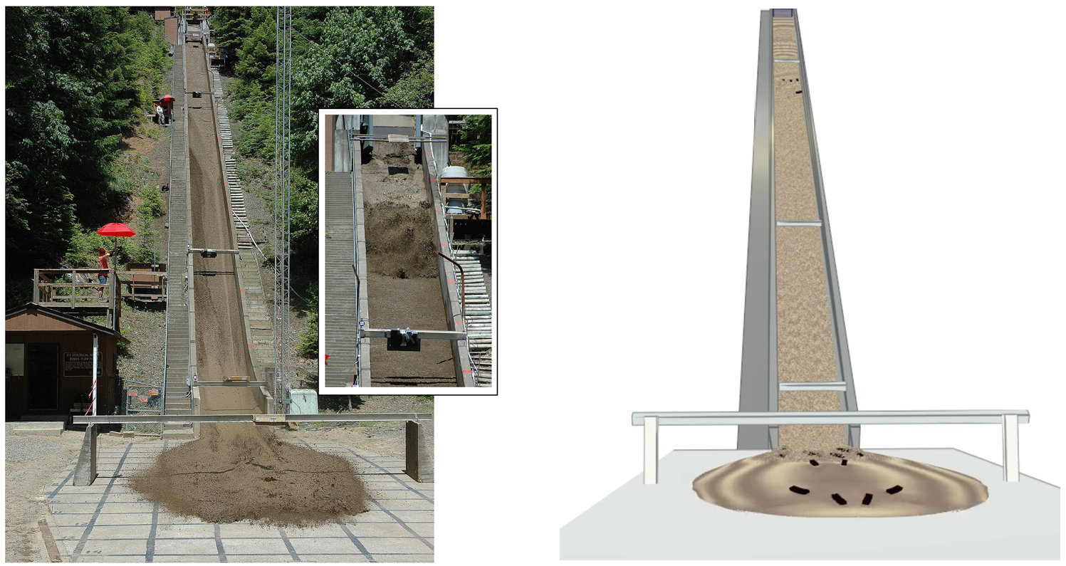
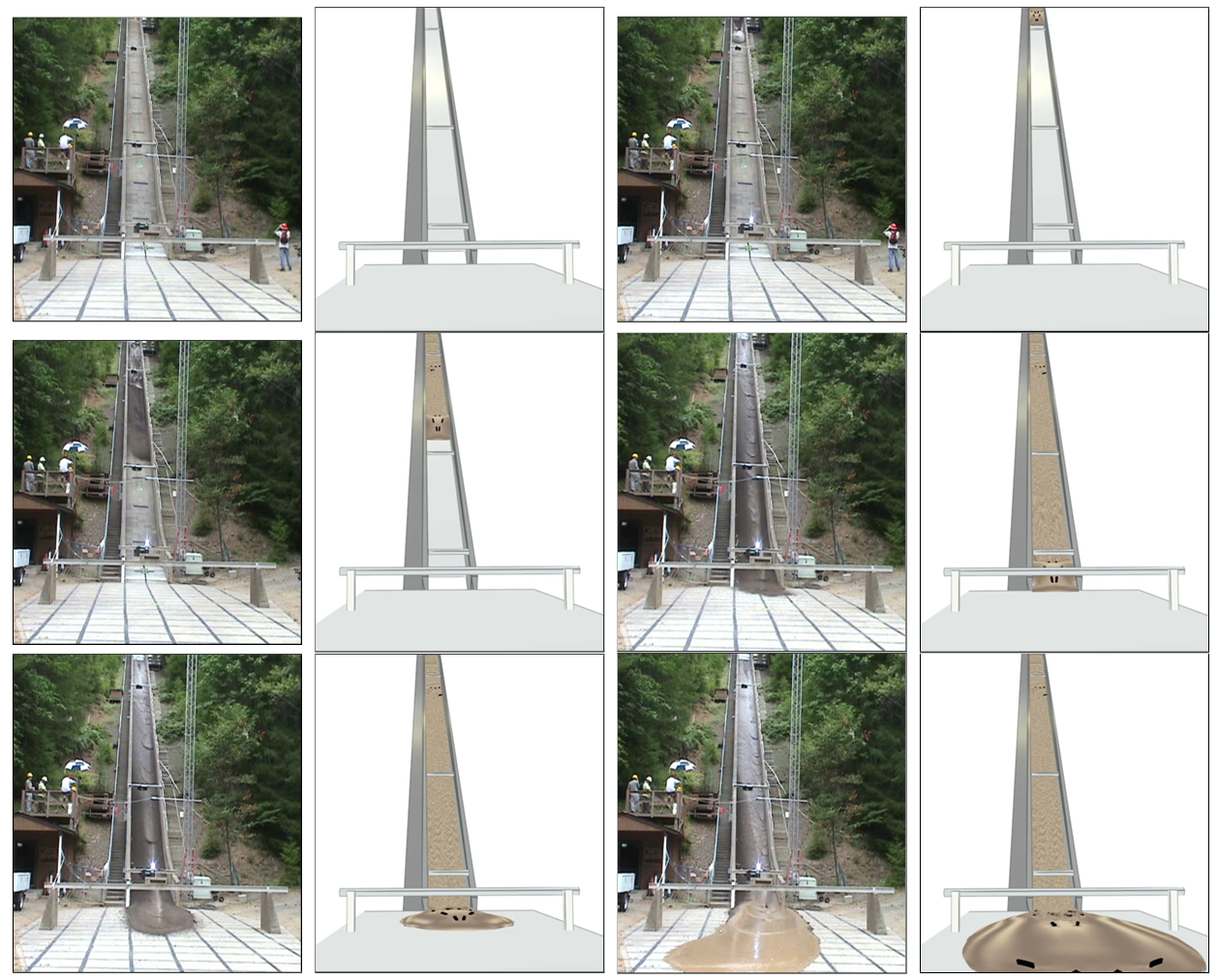
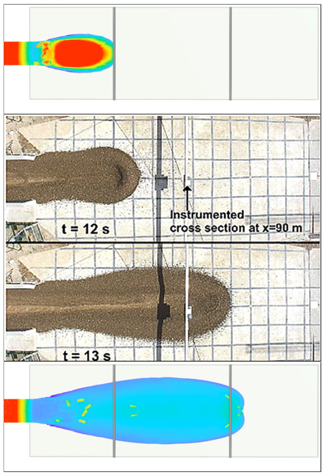
Fig. 4.10.1.3 Comparison of experimental and simulation results at high resolution.
On a final note before proceeding to describe the whole HydroUQ workflow, we remind the reader that our workflow aims to study structural response under extreme debris-flow loads at a reduced scale. The original experiments did seek to discern pressure trends for similar scenarios but were not truly concerned with structural loading and response, hence this represents an extrapolation of their work into a new domain.
4.10.2. Set-Up
4.10.2.1. Step 1: UQ
Configure Forward sampling to explore structural/material uncertainty under a fixed debris-flow signal traveling downslope.
Engine: Dakota
Forward Propagation: Sampling method (e.g., LHS) with
samples(e.g.,20) and a reproducibleseed(e.g.,1).
4.10.2.2. Step 2: GI
Set General Information and Units consistent with experiments (length, time, density, gravity). Record project metadata.
Structure name:
Concrete Box @ USGS Debris-Flow FlumeUnits: choose a consistent set (e.g., N-m-s or kips-in-s)
Note
Keep GI, SIM, EVT, and FEM units consistent. Match MPM’s length/time scales and OpenSees integration settings (e.g., time step). Verify any force/unit conversions used during load mapping.
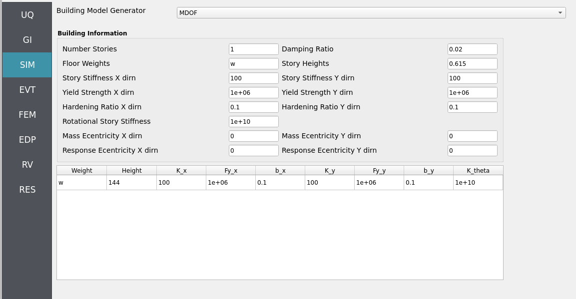
4.10.2.3. Step 3: SIM
The structural model is as follows: a single-story Multi-Degree-of-Freedom system (MDOF, see Multiple Degrees of Freedom (MDOF)) replicating a structural box placed at the base of the hillslope.
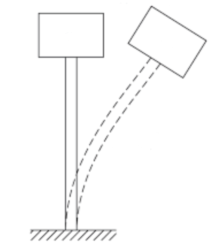
Fig. 4.10.2.3.1 Schematic of a single-story MDOF structure representing a structural box undergoing deflection from MPM derived debris-flow loading.
Note
The structure will be represented initially as a rigid boundary in MPM to recover local debris-flow forces at grid nodes for direct comparison with load-cell data. Structural dynamic response is added later by mapping these loads onto an OpenSees model defined here in the SIM panel with analysis options set in the FEM panel.
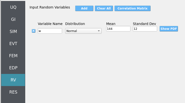
Uncertain structural properties (treated as RVs; see Step 7):
w: Weight. Mean144, stdev12
Bind parameters via setting alphabetic characters in the variable input boxes (e.g., w) so the RV panel recognizes and manages them automatically.
While not necessary to have, we show the template OpenSees model for your reference. The script generated in the backend by the MDOF module resembles the following, MDOF.tcl:
Click to expand the OpenSees input file used for this example
 1model BasicBuilder -ndm 3 -ndf 6
 2pset w 144.0
 3node 2 0 0 576 -mass $w $w  0.0  0.0  0.0  0.0
 4fix 2 0 0 1 1 1 0
 5node 1 0 0 0
 6fix 1 1 1 1 1 1 1
 7uniaxialMaterial Steel01 1 1e+06 100 0.1
 8uniaxialMaterial Steel01 2 1e+06 100 0.1
 9uniaxialMaterial Elastic 3 1e+10
10element zeroLength 1 1 2 -mat 1 2 3 -dir 1 2 6 -doRayleigh
4.10.2.4. Step 4: EVT
In this walk-through we will give a detailed step-by-step configuration of the MPM EVT module.
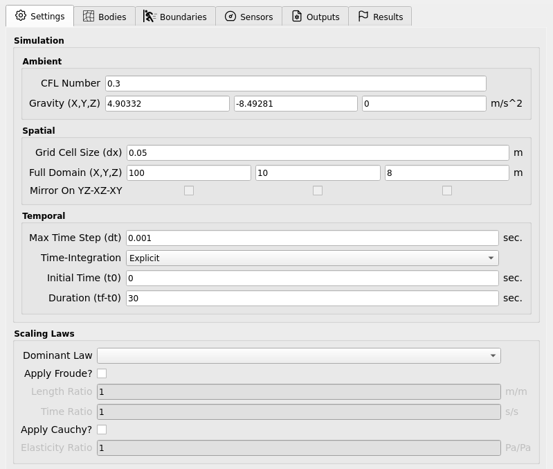
Settings
Open Settings. Here we set the simulation time, the time step, and the grid resolution, among other pre-simulation decisions. Note that we have rotated the gravity vector to digitally create the 31 degree hill-slope out of an otherwise horizontal plane.
Bodies
Geometry
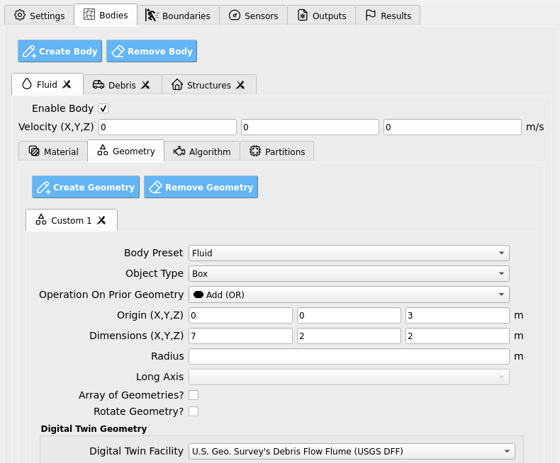
Fluid geometry
Open Bodies / Fluid / Geometry. Here we set the geometry of the flume’s sand-mass. Note that it is simply a rectangular prism located at the top of the hillslope, where it is ready to collapse under gravity.
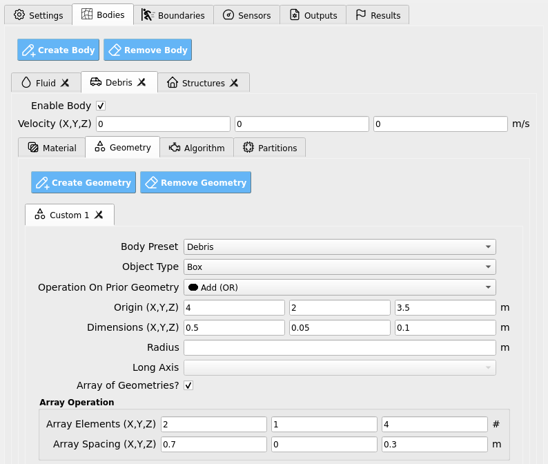
Debris geometry:
Open Bodies / Debris / Geometry. Here we set the debris properties, such as the number of debris, the size of the debris, and the spacing between the debris. Rotation is another option, though not used in this example. We’ve elected to use an 4 x 2 grid of debris (longitudinal axis parallel to long-axis of the flume).
Material
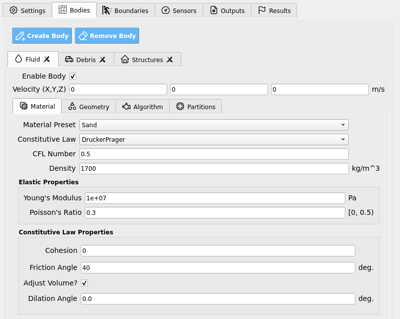
Fluid material:
Open Bodies / Fluid / Material. Here we set the material properties of the sand. We base values off of those reported for the dry specimen in [Iverson2016] and assume that a standard Drucker-Prager constitutive model is applicable.
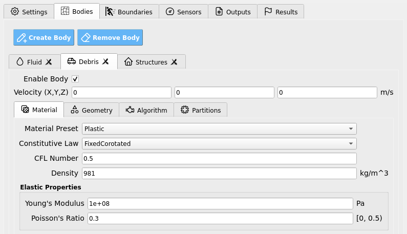
Debris material:
Moving onto the creation of an ordered debris array, we set the debris properties in the Bodies / Debris / Material tab. We will assume debris are made of HDPE plastic so that they remain mostly buoyant while entrained in the debris-flow. This also helps to match the extensive literature on tsunami debris which uses HDPE plastic debris, as seen in Lewis 2023 [Lewis2023], Mascarenas 2022 [Mascarenas2022], and Shekhar et al. 2020 [Shekhar2020].
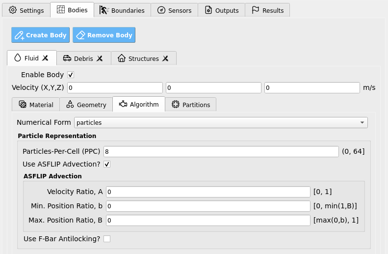
Algorithm
Open Bodies / Fluid / Algorithm. Here we set the sand algorithm parameters for the simulation. This is an advanced feature of the MPM module, it is best not to alter it too much. We choose not to apply F-Bar antilocking as our sand is not numerically stiff enough to require it. The associated toggle must be unchecked. ASFLIP is turned on to allow us to apply friction to the sand mass as it flows downslope, as well as to allow us to track its velocity on a per-particle basis.
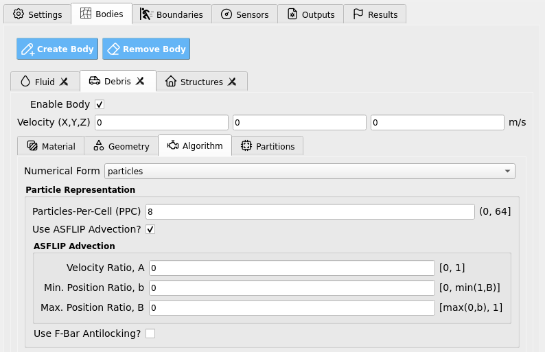
In Bodies / Debris / Algorithm we set debris as follows: ASFLIP is turned on and F-Bar antilocking is turned off. Turning on ASFLIP is, again, for the purpose of applying friction to the debris when appropriate (i.e., when contacting the flume floor) and for tracking debris particle velocity vectors.
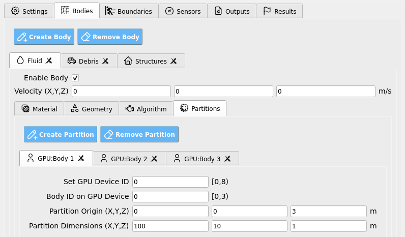
Partitions:
Open Bodies / Fluid / Partitions. This is an advanced feature of the MPM module which allows us to partition material bodies across hardware devices to optimize simulations. These may be kept as their default values, which have already been set for compatibility on the remote HPC system.
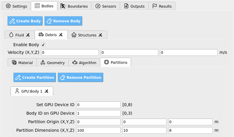
Next, Bodies / Debris / Partitions defines a partition where the debris may exist in our flume domain and defines the hardware device (i.e., GPU) that they will be simulated on. Keep this as the default unless you are an advanced user.
Structure:
Finally, open Bodies / Structures. Uncheck the box that enables this body. We will not model the structure as a deformable MPM material body in this example, instead, we will approximate it as a rigid MPM boundary a few steps from now. After the MPM simulation we will map loads from the boundary to an OpenSees structure for structural analysis, see Steps 3 and 5 for configuration.

Fig. 4.10.2.4.1 HydroUQ Bodies Structures GUI
Boundaries
Wave Flume boundary:
Open Boundaries / Flume Facility. We will set the flume boundary to be a rigid body, with a fixed separable velocity condition. Bathymetry joint points should be identical to the ones used in Bodies / Fluid / Geometry. Large friction coefficients of 2 are applied to replicate sand on concrete. Note that you may increase these in the range of 5 - 20 to try to better replicate the macro-roughness of the bumpy hillslope and runout pads used in experiments.
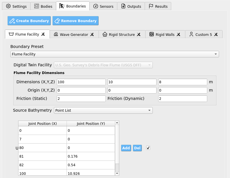
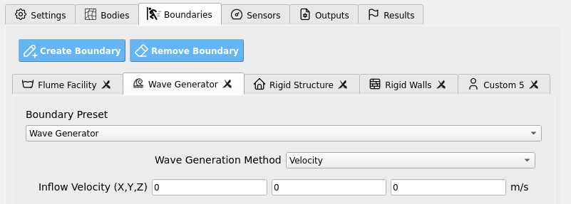
Wave Generator:
Open Boundaries / Wave Generator. As our so-called wave-generation method is the application of gravity to a sand-mass, we simply need to move the wave generator boundary condition outside of our digital flume so that it doesn’t interfere with the debris-flow. It may also be removed entirely, if desired.
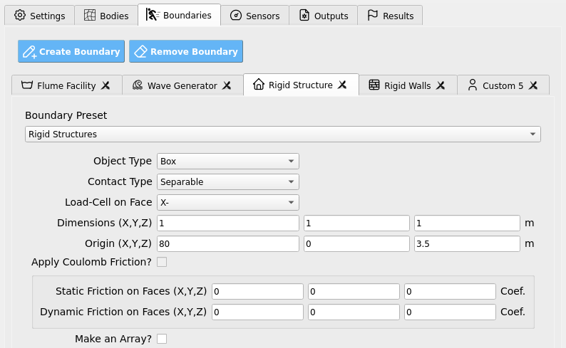
Rigid Structure:
Open Boundaries / Rigid Structure. This is where we will specify the structure as a boundary condition. By doing so, we can determine the exact loads on the rigid boundary grid-nodes, which automatically map to the model defined in the SIM and FEM tab in Steps 3 and 5 for potentially nonlinear UQ structural response analysis.
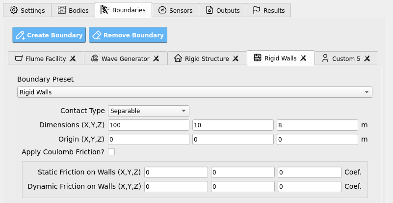
Rigid Exterior Walls:
Open Boundaries / Rigid Walls. Set to encompass the flume domain and runout pad.
Side Walls
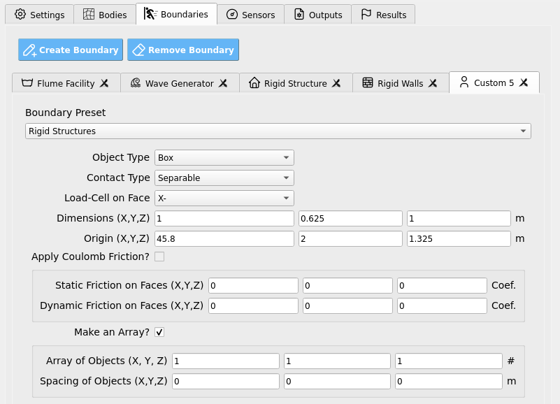
Click Create Boundary. Navigate to Boundaries / Custom 5. This boundary will be used to define the side-walls of the flume experiments. Define them as rigid rectangular prisms as below in an array of two, with a gap inbetween designated for the downslope debris-flow development.
Sensors
Wave Gauges:
Open Sensors / Wave Gauges. Set the Use these sensor? box to True so that the simulation will output results for the instruments we set on this page.
Four wave gauges will be defined along the hillslope ramp’s path towards the structural face, where we anticipate a sand buffer to develop.
Set the origins and dimensions of each wave gauge to encompass at least one grid-cell in each direction as in the table below. To match experimental conditions, we also apply a 30 Hz sampling rate to the wave gauges.
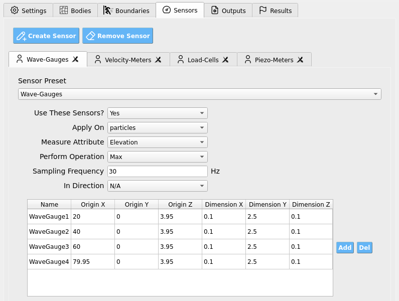
These wave gauges will read all numerical bodies (i.e. particles) within their defined regions at every sampling step and will report the highest elevation value (Position Y) of a contained body as the free-surface elevation at that gauge. The results are written into our sensor results files which we will later analyze.
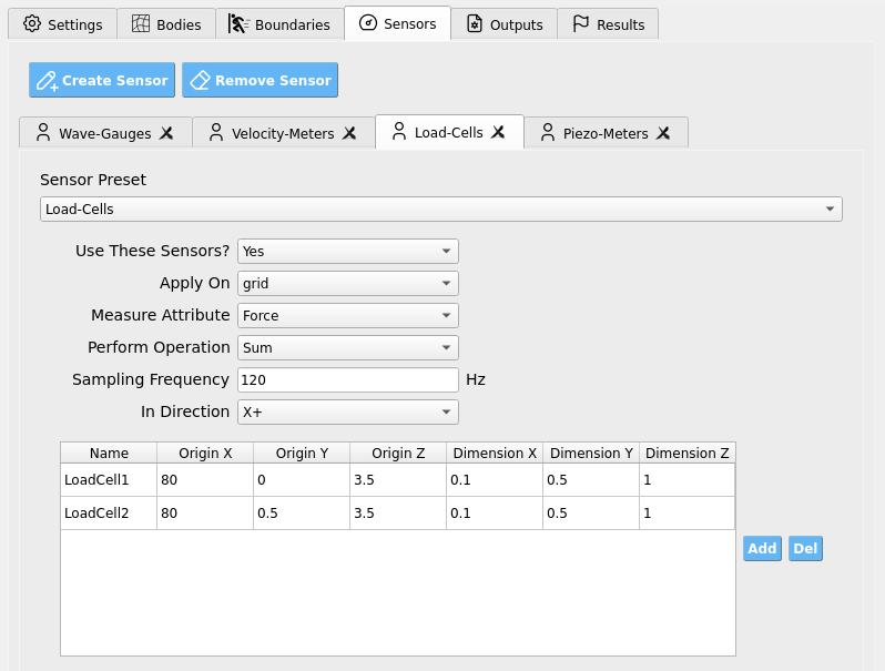
Load Cells:
Open Sensors / Load Cells. Set the Use these sensor? box to True so that the simulation will output results for the instruments we set on this page. Two load cells are defined so that we may map loads onto two nodes of our OpenSees structural model which we defined in Steps 3 and 5. Output frequency is set to 120 Hz to capture primary load phenomena, but note that the experiments themselves did not feature such load-cells.
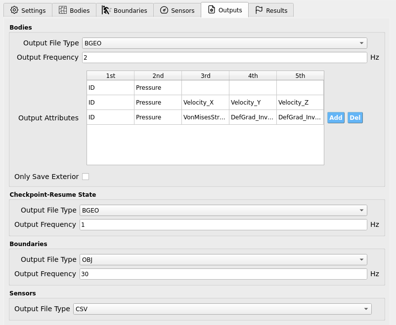
Outputs
Open Outputs. Here we set the non-physical output parameters for the simulation, e.g. attributes to save per frame and file extension types. The particle bodies’ output frequency is set to 2 Hz, meaning the simulation will output results every 0.5 seconds. This is to save disk space and reduce I/O load, but it may be increased if you wish to make animations (e.g., 10 - 30 Hz). Fill the rest of the data in the figure into your GUI to ensure all your outputs match this example. You may alter output attributes if you are an advanced user familiar with ClaymoreUW attributes and wish to perform more advanced analysis.
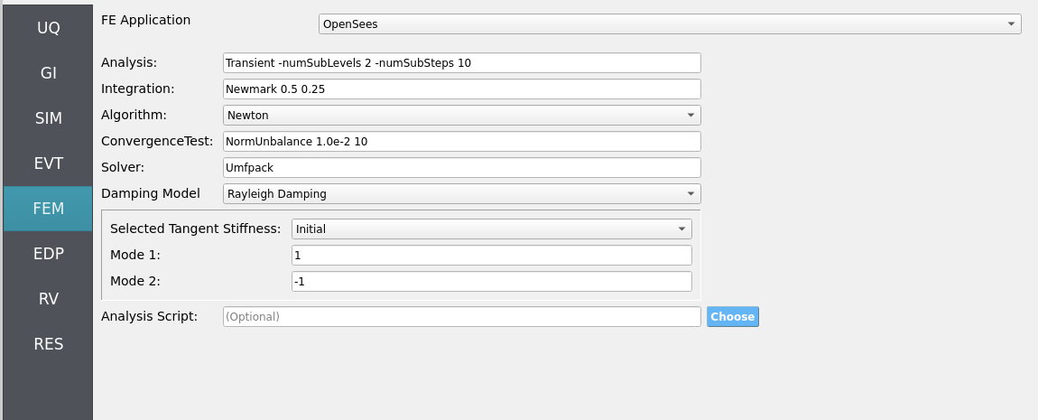
4.10.2.5. Step 5: FEM
This example insofar focused on debris-flow forces measured on rigid structures. To perform true structural response analysis, map recovered boundary loads to an OpenSees model in SIM and configure dynamic analysis here as in other HydroUQ tutorials.
Solver: OpenSees dynamic analysis. Check:
Integration step compatible with MPM sensor output interval.
Algorithm/convergence tolerances suitable for expected nonlinearity.
Damping model as needed (e.g., Rayleigh).
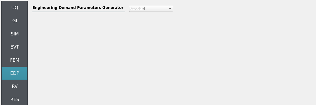
4.10.2.6. Step 6: EDP
Select Engineering Demand Parameters (EDPs) to summarize response:
Peak Floor Acceleration (PFA)
Root Mean Square Acceleration (RMSA)
Peak Floor Displacement (PFD)
Peak Interstory Drift (PID)
Note that other quantities of interest (QoI) are theoretically obtainable from HydroUQ, if the custom EDP module is configured. E.g.:
Wave: free-surface elevation η(t) at gauges.
Debris motion: longitudinal displacement (forward/back), lateral spreading angle, stack interaction metrics (contact counts/overturns).
Loads: obstacle force time histories (impact peaks, impulses).
4.10.2.7. Step 7: RV
Define distributions for structural RV:
Structural
w: Normal (mean144, stdev12)
For future UQ, consider:
Debris: mass variance, friction coefficients (debris-apron, debris-debris).
Wave: amplitude/period tolerance relative to vacuum-maker target.
Obstacles: small misalignment/placement tolerance.
4.10.3. Simulation
This case was executed on TACC Stampede3 using 2x NVIDIA H100 GPUs on a single node (queue: h100).
Simulated physical time: 15 seconds. Wall time: 90 minutes (allow ample Max Run Time in job settings).
Important
Provide generous Max Run Time, on the order of 60 to 90 minutes, to complete the run and post-processing before scheduler limits are reached.
Warning
Keep sensor regions, counts, sampling rates, and output frequencies reasonable—excess I/O can dominate runtime.
Outputs
Sensor CSVs (gauges, debris CoM, loads) at your chosen rates.
Particle/field snapshots (e.g., BGEO/VTK) for visualization/diagnostics.
4.10.4. Analysis
Accessing Results and Simulation Files
When the simulation job has been completed, the results and simulation files will be available on the remote system for retrieval or remote post-processing.
Retrieving the results.zip, templatedir.zip, workdir.tar.gz, and MPM folders will allow you to analyze all of the simulation output (e.g., hydrodynamic, structural, uncertainty quantification).
results.zip: Contains primary uncertainty quantification output and MPM sensor files. This will be the primary place for analysis.templatedir.zip: Contains template and workflow files for the job. This is an important resource for debugging your workflows.workdir.tar.gz: Contains the working directories in which each unique simulation was ran. This is where structural response uncertainty is expanded on typically.MPM: Contains all the MPM simulation files. Includes the raw particle output frames which can be used to create animations or to perform more advanced post-processing.
The most straightforward way to retrieve the most important files, results.zip and templatedir.zip, is by clicking the GET From DesignSafe button in HydroUQ.

Fig. 4.10.4.1 HydroUQ GET From DesignSafe button, which opens up a jobs table of all your remote simulations.
Then, right-click on your job (if it is finished) and select Retrieve Data. This will download results.zip and templatedir.zip.
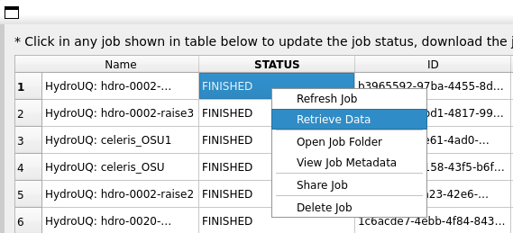
Fig. 4.10.4.2 Locating the Retrieve Data button in the HydroUQ remote jobs table.
HydroUQ will then automatically unzip them into results and templatedir, which will be located in {your_path}/HydroUQ/RemoteWorkDir/tmp.SimCenter. On most systems, this will be ~/Documents/HydroUQ/RemoteWorkDir/tmp.SimCenter, but you can check by clicking on Files / Preferences on the upper-left corner of HydroUQ.
To retrieve workdir.tar.gz and MPM, there are two approaches:
You can right-click on your job within HydroUQ and select
Open Job Folderto be taken directly to the Design Safe web-page displaying all remote files.
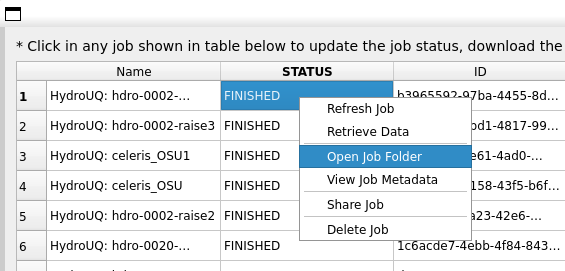
Fig. 4.10.4.3 Locating the Open Job Folder button in the HydroUQ remote jobs table.
You can manually navigate to the designsafe-ci.org website. For the latter, login and go to
Upper-right Drop-down/Job Status.

Fig. 4.10.4.4 Locating the job files on DesignSafe
Check if the job has finished in the central vertical drawer by refreshing the page. If it has, click View Details.
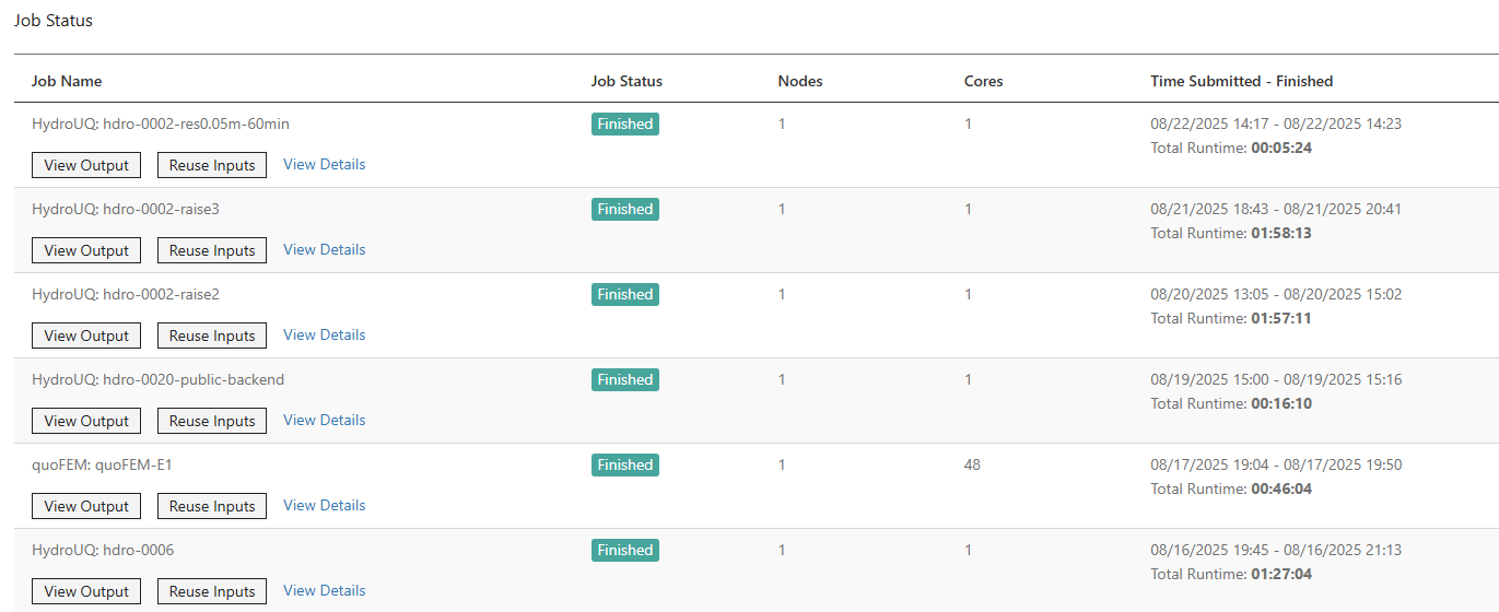
Fig. 4.10.4.5 Job status is finished on DesignSafe
Once the job is finished, the output files should be available in the directory which the analysis results were sent to
Find the files by clicking View Output.
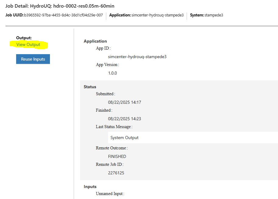
Fig. 4.10.4.6 Viewing the job files on DesignSafe
After navigating to your job folder by one of two ways, it is time to move files for processing. Move important files to somewhere in My Data/ for easier processing. Use the extractor tool available on DesignSafe to unzip the results.zip, workdir.tar.gz, and templatedir.zip folders natively on DesignSafe.
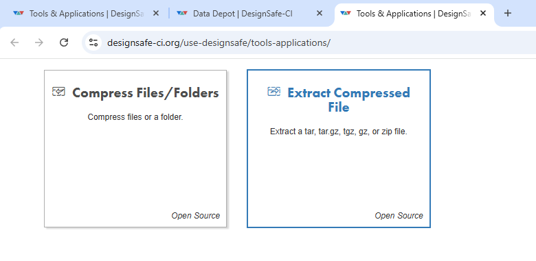
Fig. 4.10.4.7 Extracting the results.zip folder on DesignSafe
Alternatively, you may directly download the zipped folders to your PC, which will require you to use the DesignSafe zip tool on the MPM folder prior.
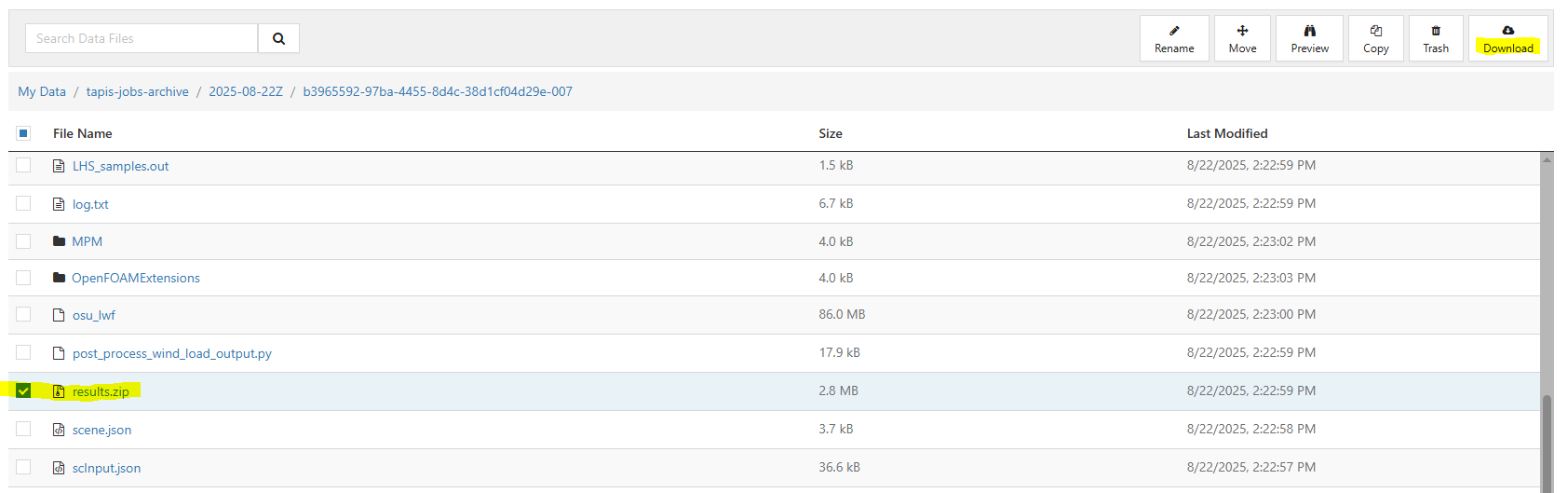
Fig. 4.10.4.8 Download button on DesignSafe shown in red
Locate the downloaded zip folders and extract them somewhere convenient. The HydroUQ local or remote work directory on your computer is a good option.
Warning
Files in the HydroUQ local and remote working directories may be erased if another simulation is set up in HydroUQ, so keep a backup if you wish to maintain the files.
Particle geometry files often have a BGEO extension and are located in the MPM folder. Open with Side FX Houdini Apprentice (free to use) to look at MPM results in high-detail, or use the PartIO library.
HydroUQ’s sensor/probe/instrument output is available in {your_path}/HydroUQ/RemoteWorkDir/tmp.SimCenter/results/ as CSV files. You may process these files as you wish, most opt to use custom Python scripts or Excel due to their simplicity.
Note
For convenience, HydroUQ also includes basic plotting of all sensors files in the EVT / Results tab. Click Post-Process Sensors, configure the drop-down boxes for the sensor you wish to view, and then click Plot.
Plotting the wave gauges shows the development of a debris-flow as it propagates from the initial hill-perched mass down the highly frictional hillslope. It attains a steady-state flow-depth of approximately 0.25 meters prior to collision with the rigid structural box, which causes a ‘splash’ upto 2.5 meter which settles down to approximately 0.75 to 1.0 meter of quasi-hydrostatic sand-mass build-up at the structural face.
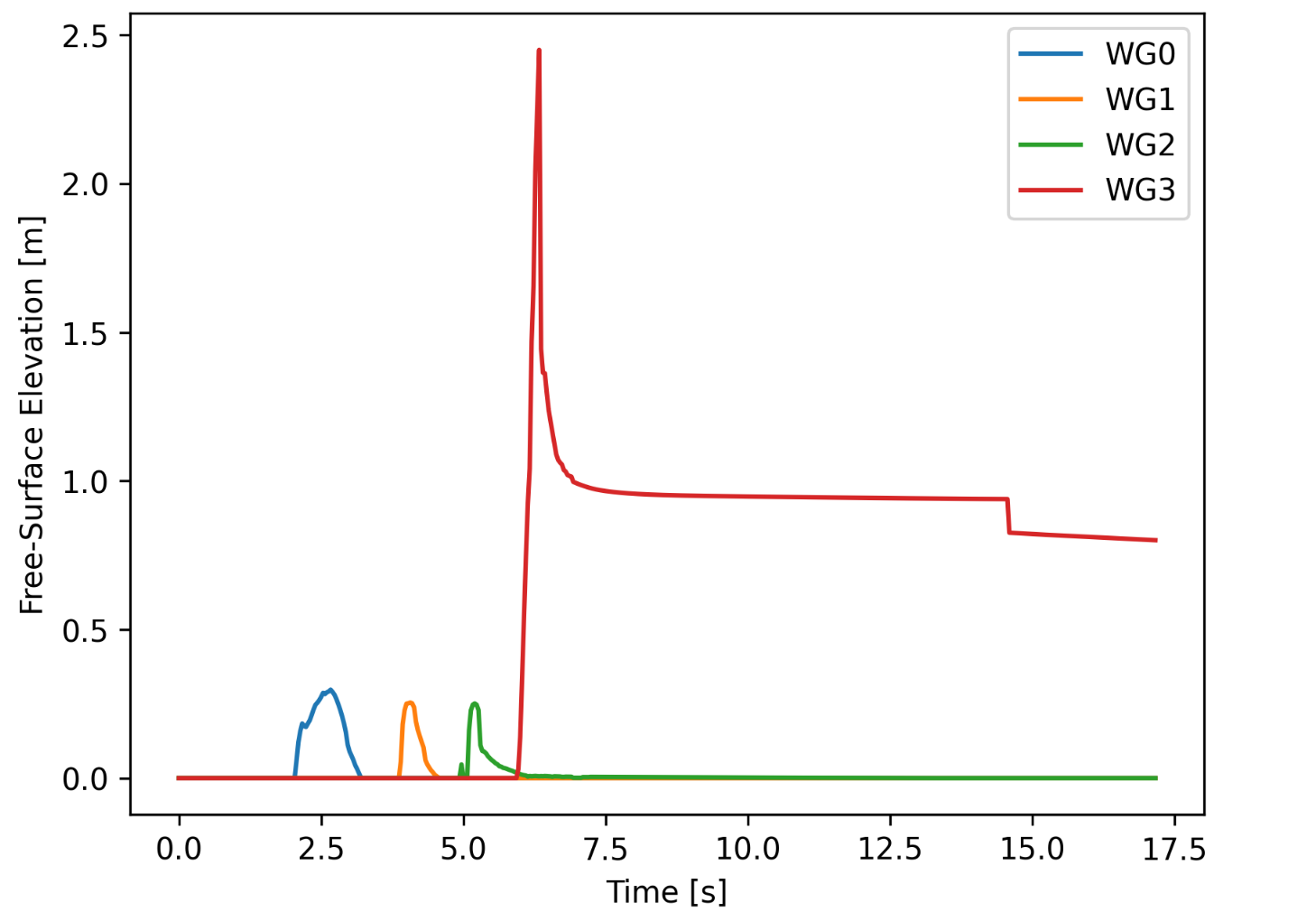
Fig. 4.10.4.9 Simulated free-surface elevations at four wave gauges in MPM.
Load-cell data shows an initially extremely high peak force caused by the kinematic energy transfer of the fast moving debris-flow. It is followed by decaying damming forces and eventually just a slight quasi-hydrostatic loading. These results emphasize the extreme hazard that fast moving debris-flow pose to structures, even at this reduced scale.
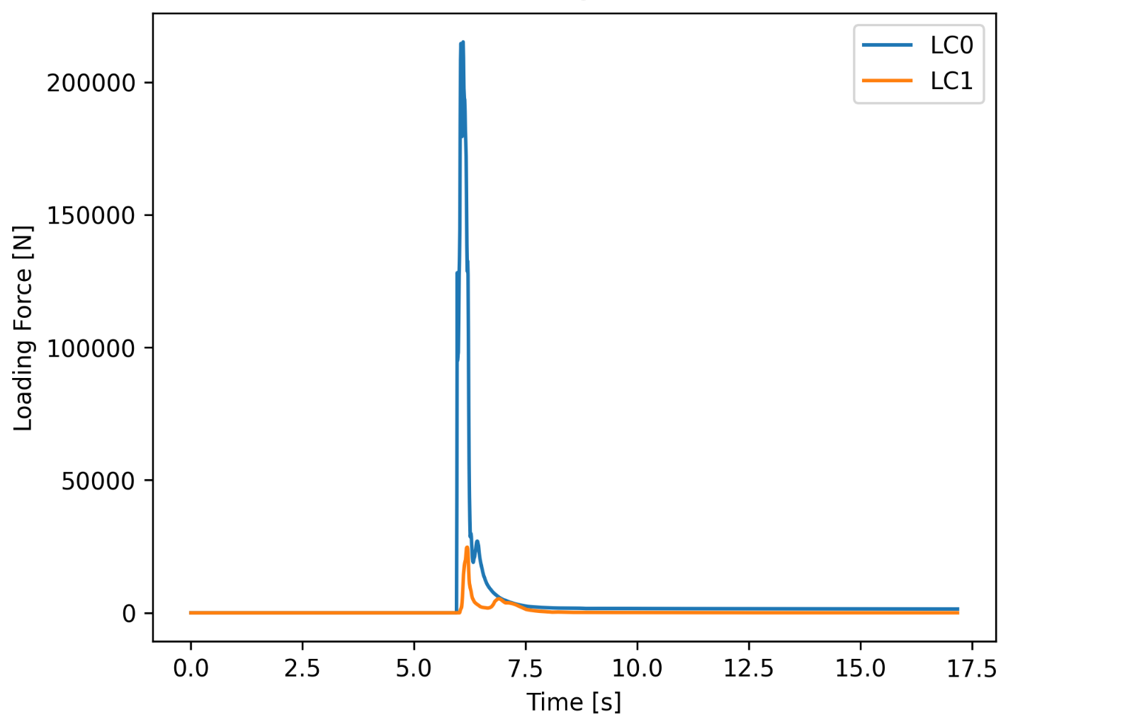
Fig. 4.10.4.10 Simulated load-cell forces in MPM. These are later mapped onto an OpenSees structure for dynamic response analysis.
To demonstrate the applicability of the MPM module within HydroUQ to replicating these experiments, we show below a higher resolution case from [Bonus2023Dissertation] which replicates many aspects of even a partially liquefied flow. For an ever more apt comparison, a side-by-side of dry experiments and simulations is also shown in the overview section.
Elevation contours of the runout can also be visualized as seen below. This shows appropriate kinetic energy dissipation as the debris-flow propagates down the frictional hillslope and onto the frictional runout pad. High relative accuracy in the runout pattern also suggests that the Drucker-Prager constitutive model was an appropriate choice for the dry experimental scenario examined.
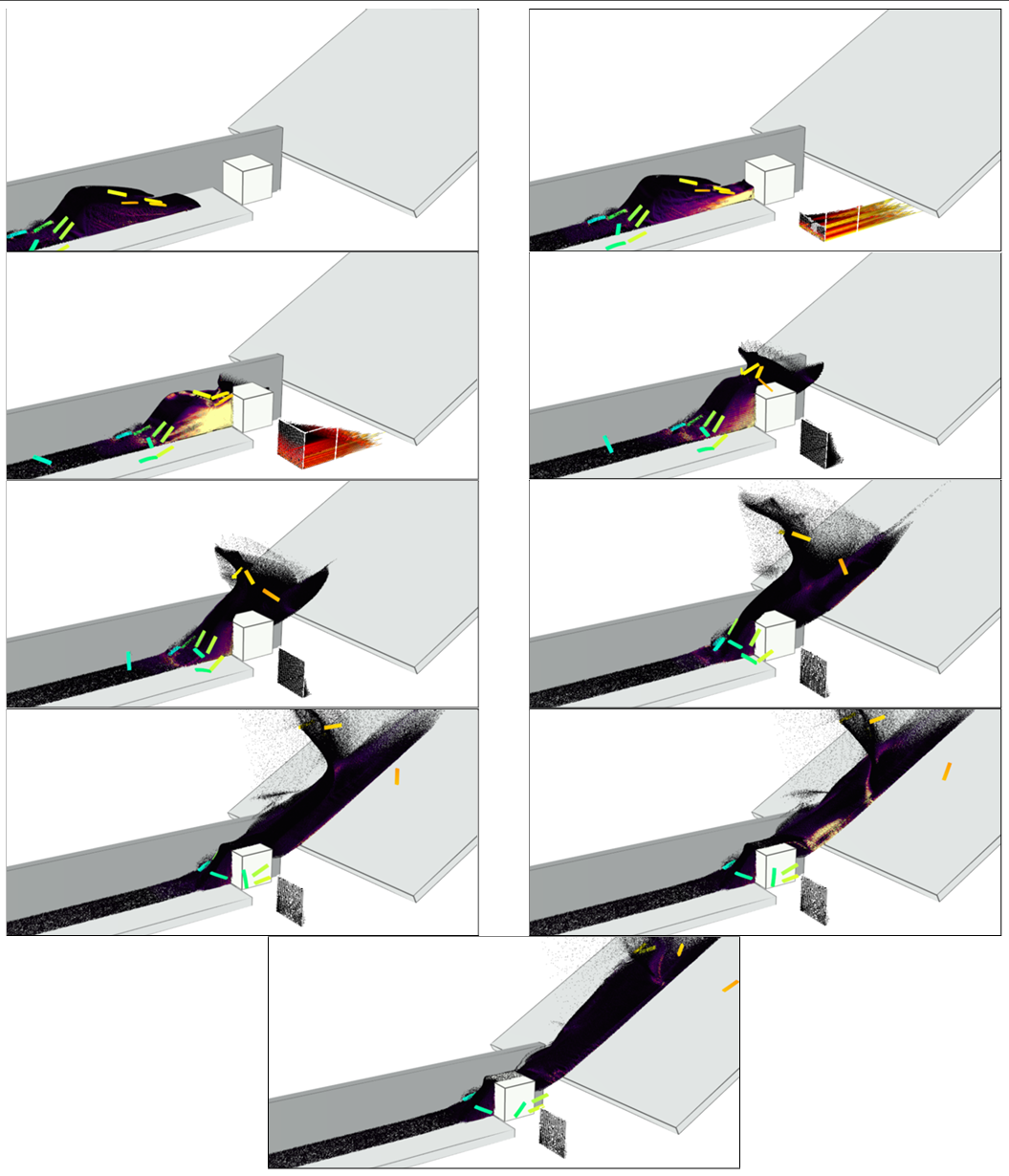
Finally, the impact on the structural box can be looked at more closely. Here we see the pressure visualized in the debris-flow with entrained debris color-coded for visual identification. A clear build-up of mass and pressure at the structure is observed, followed by a ‘splash’ dissipating remaining energy, and finally a quasi-hydrostatic state is reached at the structural face. Debris are seen to flow with and decouple from the debris-flow without issue.
Structural Analysis
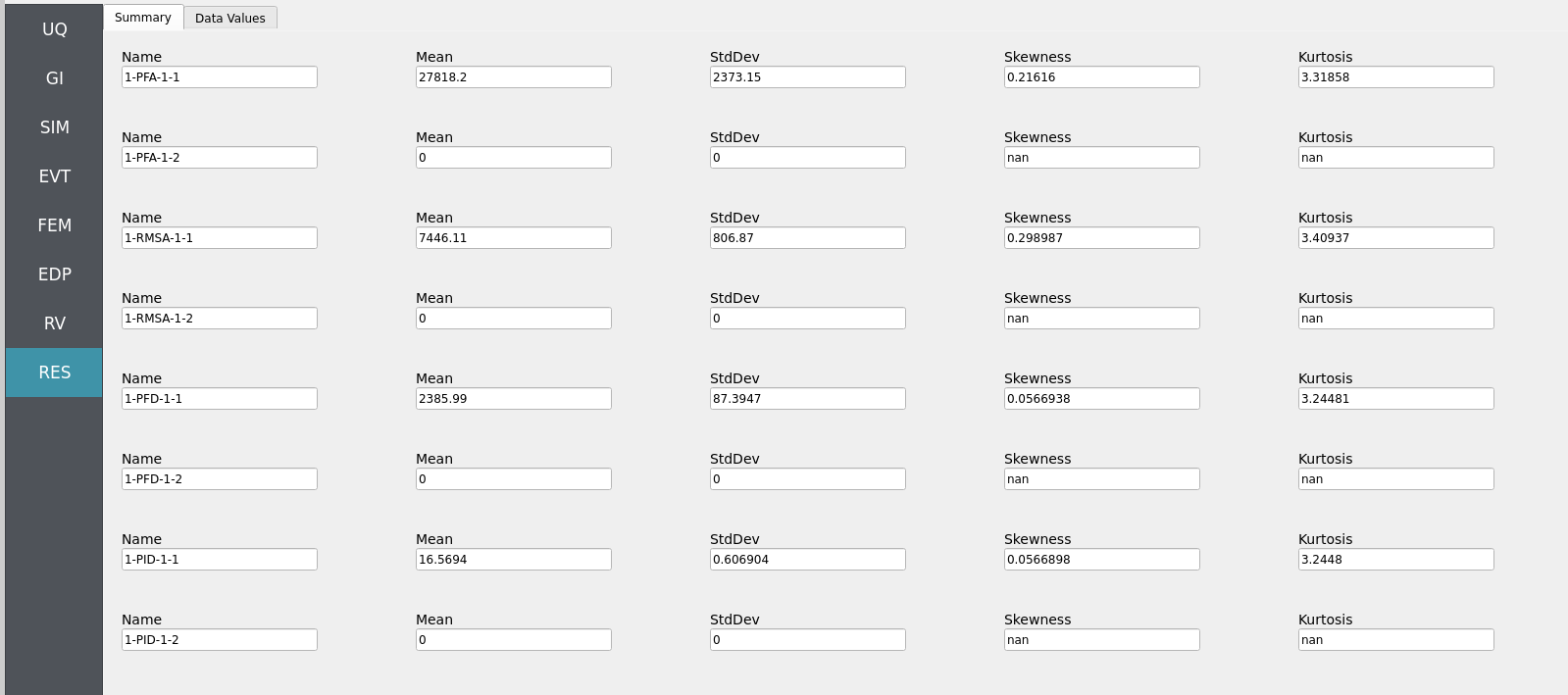
Returning to our primary HydroUQ workflow, which concerns uncertainty in structural response, we may now view the final results in the RES tab. Clicking Summary on the top-bar, a statistical summary of results is shown below:
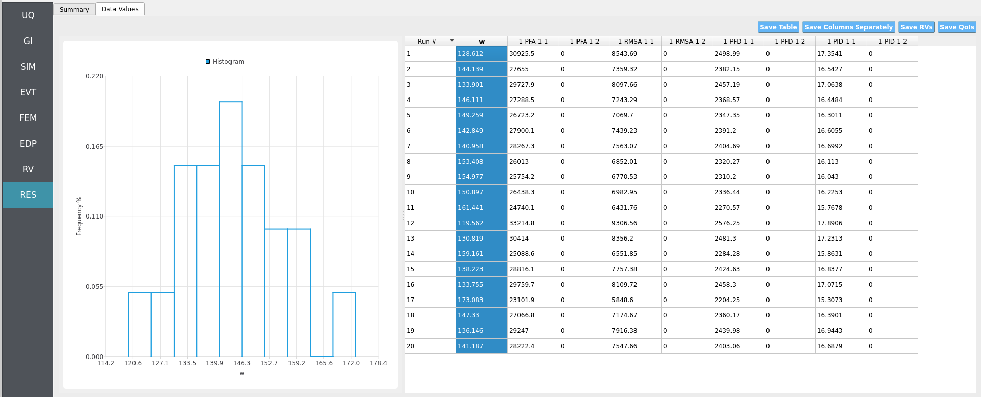
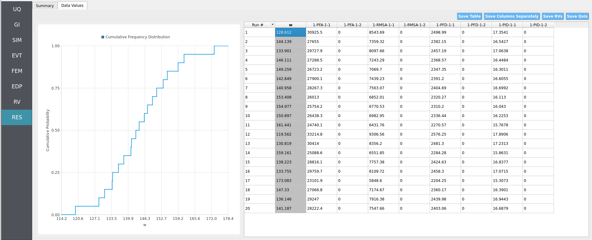
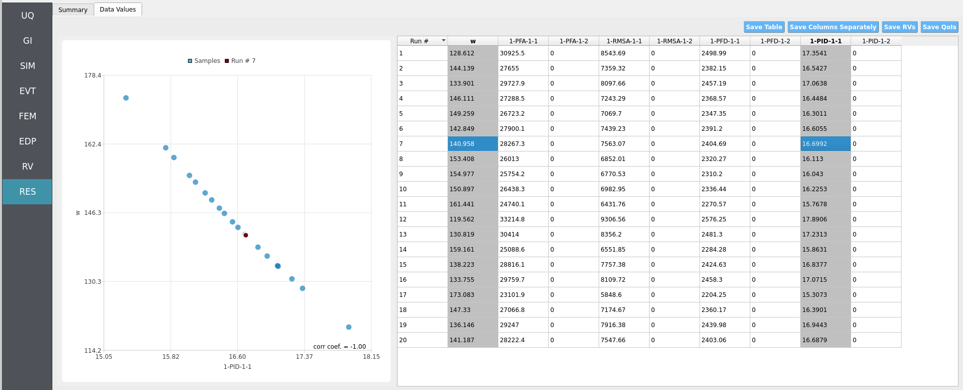
Clicking Data Values on the top-bar shows detailed histograms, cumulative distribution functions, and scatter plots relating the dependent and independent variables:
Note
In the Data Values tab, left- and right-click column headers to change plot axes; selecting a single column with both clicks displays frequency and CDF plots.
Note
Use consistent Froude similitude scaling when comparing numerical simulations, experiments, and full-scale scenarios. For cross-method comparisons, adopt identical debris footprints, friction models, probe placement, and other pertinent parameters to reduce bias.
For more advanced analysis, export results as a CSV file by clicking Save Table on the upper-right of the application window. This will save the independent and dependent variable data. I.e., the Random Variables you defined and the Engineering Demand Parameters determined from the structural response per each simulation.
To save your simulation configuration with results included, click File / Save As and specify a location for the HydroUQ JSON input file to be recorded to. You may then reload the file at a later time by clicking File / Open. You may also send it to others by email or place it in an online repository for research reproducibility. This example’s input file is viewable at Reproducibility.
To directly share your simulation job and results in HydroUQ with other DesignSafe users, click GET from DesignSafe. Then, navigate to the row with your job and right-click it. Select Share Job. You may then enter the DesignSafe username or usernames (comma-separated) to share with.
Important
Sharing a job requires that the job was initially ran with an Archive System ID (listed in the GET from DesignSafe table’s columns) that is not designsafe.storage.default. Any other Archive System ID allows for sharing with DesignSafe members on the associated project. See Jobs for more details.
4.10.5. Conclusions
The HydroUQ MPM runs of the digital USGS DFF reproduce the mechanistic signatures of a dry debris-flow highlighted in the experiments by [Iverson2016]. In summary:
The model captures appropriate depth-velocity flow pairing relative to the sand material and frictional hillslope.
Against a vertical barrier, runup is shock-dominated: front thickening, rapid momentum loss, and a clear pressure/impulse peak followed by brief quasi-static damming.
The ab initio (dry, high-friction) configuration provides a conservative lower bound on runup for comparable geometries if investigating dry, high-friction scenarios.
Runout is reasonably captured relative to the macro-friction of the bumpy hillslope and runout pads that are replicated with a large Coulomb friction coefficient.
Further, we extrapolate to structural analysis by mapping MPM-derived loads onto an OpenSees model in our modular workflow, allowing for design insights to be garnered if analysis is refined.
For HydroUQ users interested in advanced analysis of further cases in this experimental set and digital flume, we may suggest investigating:
When the barrier is conceptualized with an adverse slope (parametric variants), do the runs show a pre-shock mass/momentum transfer to the front that increases runup before a shock forms, i.e., consistent with the sloping-obstacle observations of experiments?
Do predicted runup height scales with \(Fr\) at the toe and decreases with increasing basal \(\mu_{\mathrm{eff}}\), matching the trend that less-liquefied flows run up less?
Whether data-informed variants (calibrated \(Fr\), \(h_f\), \(\mu_{\mathrm{eff}}\), or adding a pore-pressure mechanism) improve quantitative accuracy without changing the underlying shock vs pre-shock narrative?
Does the model resolve flow redirection and reflected-wave growth, which feed back on the incoming body to modulate the impulse tail? Do these multidimensional effects explain why simplified analytical models can bracket but not fully match peak loads in all regimes?
Report \(Fr\), \(h_f\), \(U_f\) at a fixed station upstream; plot runup ratio \(R/h_f\) vs \(Fr\) and vs \(\mu_{\mathrm{eff}}\) and evaluate trends.
Integrate wall-normal force to obtain impulse; separate peak and damming contributions using a suitable decomposition method.
Visualize thickness jumps and reflected waves (space-time plots at the wall and along the pad) to diagnose shock onset.
For design-leaning studies, map the envelope of \((Fr, \mu_{\mathrm{eff}})\) to runup and impulse fragility curves, then propagate uncertainty with Forward UQ.
Explore use of more advanced UQ techniques for refined structural design in this extreme loading environment.
Overall, the MPM digital flume captures the physics that matter for runup forecasting — shock formation, flux-front coupling, and friction-controlled dissipation — and offers a clear path to higher fidelity (two-phase coupling, explicit roughness) when needed. This supports using HydroUQ MPM as a predictive, mechanistic tool for evaluating debris-flow runup and impact loads on protective structures across a spectrum of flow regimes.
4.10.6. References
Iverson, R. M., Logan, M., LaHusen, R. G., & Berti, M. (2010). The perfect debris flow? Aggregated results from 28 large-scale experiments. Journal of Geophysical Research F: Earth Surface, 115(F3), F03005-. https://doi.org/10.1029/2009JF001514
Iverson, R. M., George, D. L., & Logan, M. (2016). Debris flow runup on vertical barriers and adverse slopes. Journal of Geophysical Research: Earth Surface, 121(12), 2333–2357. https://doi.org/https://doi.org/10.1002/2016JF003933
Bonus, Justin (2023). “Evaluation of Fluid-Driven Debris Impacts in a High-Performance Multi-GPU Material Point Method.” PhD thesis. University of Washington, Seattle.
Bonus, J., & Arduino, P. (2025). ClaymoreUW. Zenodo. https://doi.org/10.5281/zenodo.15128706
4.10.7. Reproducibility
Random seed(s):
1(set in UQ)App version: HydroUQ v4.2.0 (or current)
Solver: MPM (ClaymoreUW, multi-GPU)
Hardware: TACC Lonestar6 or Stampede3, 3x A100 or 4x H100 (single node,
gpu-a100orh100queue)Simulated time: 30 seconds; Wall time: 1-2 hours
Sensor sampling: wave-gauges 120 Hz; particle output 2-10 Hz
Input: The HydroUQ input file is as follows: input.json , is used:
Click to expand the HydroUQ input file used for this example
1{
2 "Applications": {
3 "EDP": {
4 "Application": "StandardEDP",
5 "ApplicationData": {
6 }
7 },
8 "Events": [
9 {
10 "Application": "MPM",
11 "ApplicationData": {
12 },
13 "EventClassification": "Hydro",
14 "defaultMaxRunTime": "1440",
15 "driverFile": "sc_driver",
16 "inputFile": "scInput.json",
17 "maxRunTime": "120",
18 "programFile": "osu_lwf",
19 "publicDirectory": "./"
20 }
21 ],
22 "Modeling": {
23 "Application": "MDOF_BuildingModel",
24 "ApplicationData": {
25 }
26 },
27 "Simulation": {
28 "Application": "OpenSees-Simulation",
29 "ApplicationData": {
30 }
31 },
32 "UQ": {
33 "Application": "Dakota-UQ",
34 "ApplicationData": {
35 }
36 }
37 },
38 "DefaultValues": {
39 "driverFile": "driver",
40 "edpFiles": [
41 "EDP.json"
42 ],
43 "filenameAIM": "AIM.json",
44 "filenameDL": "BIM.json",
45 "filenameEDP": "EDP.json",
46 "filenameEVENT": "EVENT.json",
47 "filenameSAM": "SAM.json",
48 "filenameSIM": "SIM.json",
49 "rvFiles": [
50 "AIM.json",
51 "SAM.json",
52 "EVENT.json",
53 "SIM.json"
54 ],
55 "workflowInput": "scInput.json",
56 "workflowOutput": "EDP.json"
57 },
58 "EDP": {
59 "type": "StandardEDP"
60 },
61 "Events": [
62 {
63 "Application": "MPM",
64 "EventClassification": "Hydro",
65 "example": "USGS DFF",
66 "bodies": [
67 {
68 "algorithm": {
69 "ASFLIP_alpha": 0,
70 "ASFLIP_beta_max": 0,
71 "ASFLIP_beta_min": 0,
72 "FBAR_fused_kernel": false,
73 "FBAR_psi": 0.0,
74 "ppc": 8,
75 "type": "particles",
76 "use_ASFLIP": true,
77 "use_FBAR": false
78 },
79 "geometry": [
80 {
81 "apply_array": false,
82 "apply_rotation": false,
83 "body_preset": "Fluid",
84 "facility": "U.S. Geo. Survey's Debris Flow Flume (USGS DFF)",
85 "facility_dimensions": [
86 100.0,
87 2.0,
88 8.0
89 ],
90 "fill_flume_upto_SWL": false,
91 "object": "Box",
92 "offset": [
93 0.0,
94 0.0,
95 3.0
96 ],
97 "operation": "add",
98 "span": [
99 7,
100 2,
101 2
102 ],
103 "standing_water_level": 2,
104 "track_particle_id": [
105 "0"
106 ],
107 "use_custom_bathymetry": true
108 }
109 ],
110 "gpu": 0,
111 "material": {
112 "CFL": 0.5,
113 "beta": 0.0,
114 "youngs_modulus": 1e7,
115 "poisson_ratio": 0.3,
116 "constitutive": "DruckerPrager",
117 "material_preset": "Sand",
118 "friction_angle": 40,
119 "cohesion": 0,
120 "rho": 1700
121 },
122 "model": 0,
123 "name": "fluid",
124 "output_attribs": [
125 "ID",
126 "Pressure"
127 ],
128 "partition": [
129 {
130 "gpu": 0,
131 "model": 0,
132 "partition_end": [
133 100,
134 10.0,
135 4.0
136 ],
137 "partition_start": [
138 0.0,
139 0.0,
140 3.0
141 ]
142 },
143 {
144 "gpu": 1,
145 "model": 0,
146 "partition_end": [
147 100.0,
148 10.0,
149 5.0
150 ],
151 "partition_start": [
152 0,
153 0,
154 4.0
155 ]
156 },
157 {
158 "gpu": 2,
159 "model": 0,
160 "partition_end": [
161 100.0,
162 10.0,
163 9.0
164 ],
165 "partition_start": [
166 0,
167 0,
168 8.0
169 ]
170 }
171 ],
172 "partition_end": [
173 100.0,
174 10.0,
175 4.0
176 ],
177 "partition_start": [
178 0.0,
179 0.0,
180 3.0
181 ],
182 "target_attribs": [
183 "Position_Y"
184 ],
185 "track_attribs": [
186 "Position_X",
187 "Position_Z",
188 "Pressure"
189 ],
190 "track_particle_id": [
191 0
192 ],
193 "type": "particles",
194 "velocity": [
195 0,
196 0,
197 0
198 ]
199 },
200 {
201 "algorithm": {
202 "ASFLIP_alpha": 0,
203 "ASFLIP_beta_max": 0,
204 "ASFLIP_beta_min": 0,
205 "FBAR_fused_kernel": true,
206 "FBAR_psi": 0,
207 "ppc": 8,
208 "type": "particles",
209 "use_ASFLIP": true,
210 "use_FBAR": false
211 },
212 "geometry": [
213 {
214 "apply_array": true,
215 "apply_rotation": true,
216 "array": [
217 2,
218 1,
219 4
220 ],
221 "body_preset": "Debris",
222 "facility": "U.S. Geo. Survey's Debris Flow Flume (USGS DFF)",
223 "facility_dimensions": [
224 100.0,
225 2.0,
226 8.0
227 ],
228 "fulcrum": [
229 0,
230 0,
231 0
232 ],
233 "object": "Box",
234 "offset": [
235 4.0,
236 2.0,
237 3.5
238 ],
239 "operation": "add",
240 "rotate": [
241 0,
242 0,
243 0
244 ],
245 "spacing": [
246 0.7,
247 0,
248 0.3
249 ],
250 "span": [
251 0.5,
252 0.05,
253 0.1
254 ],
255 "track_particle_id": [
256 "0"
257 ]
258 }
259 ],
260 "gpu": 0,
261 "material": {
262 "CFL": 0.5,
263 "constitutive": "FixedCorotated",
264 "material_preset": "Plastic",
265 "poisson_ratio": 0.3,
266 "rho": 981,
267 "youngs_modulus": 100000000
268 },
269 "model": 1,
270 "name": "debris",
271 "output_attribs": [
272 "ID",
273 "Pressure",
274 "Velocity_X",
275 "Velocity_Y",
276 "Velocity_Z"
277 ],
278 "partition": [
279 {
280 "gpu": 0,
281 "model": 1,
282 "partition_end": [
283 100.0,
284 10.0,
285 8.0
286 ],
287 "partition_start": [
288 0,
289 0,
290 0
291 ]
292 }
293 ],
294 "partition_end": [
295 100.0,
296 10.0,
297 8.0
298 ],
299 "partition_start": [
300 0.0,
301 0.0,
302 0.0
303 ],
304 "target_attribs": [
305 "Position_Y"
306 ],
307 "track_attribs": [
308 "Position_X",
309 "Position_Z",
310 "Pressure"
311 ],
312 "track_particle_id": [
313 0
314 ],
315 "type": "particles",
316 "velocity": [
317 0,
318 0,
319 0
320 ]
321 },
322 {
323 "algorithm": {
324 "ASFLIP_alpha": 0,
325 "ASFLIP_beta_max": 0,
326 "ASFLIP_beta_min": 0,
327 "FBAR_fused_kernel": false,
328 "FBAR_psi": 0.0,
329 "ppc": 8,
330 "type": "particles",
331 "use_ASFLIP": true,
332 "use_FBAR": false
333 },
334 "geometry": [
335 {
336 "apply_array": false,
337 "apply_rotation": false,
338 "body_preset": "Fluid",
339 "facility": "U.S. Geo. Survey's Debris Flow Flume (USGS DFF)",
340 "facility_dimensions": [
341 100.0,
342 2.0,
343 8.0
344 ],
345 "fill_flume_upto_SWL": false,
346 "object": "Box",
347 "offset": [
348 0.0,
349 0.0,
350 3.0
351 ],
352 "operation": "add",
353 "span": [
354 7,
355 2,
356 2
357 ],
358 "standing_water_level": 2,
359 "track_particle_id": [
360 "0"
361 ],
362 "use_custom_bathymetry": true
363 }
364 ],
365 "gpu": 1,
366 "material": {
367 "CFL": 0.5,
368 "beta": 0.0,
369 "youngs_modulus": 1e7,
370 "poisson_ratio": 0.3,
371 "constitutive": "DruckerPrager",
372 "material_preset": "Sand",
373 "friction_angle": 40,
374 "cohesion": 0,
375 "rho": 1700
376 },
377 "model": 0,
378 "name": "fluid",
379 "output_attribs": [
380 "ID",
381 "Pressure"
382 ],
383 "partition": [
384 {
385 "gpu": 0,
386 "model": 0,
387 "partition_end": [
388 100,
389 10.0,
390 4.0
391 ],
392 "partition_start": [
393 0.0,
394 0.0,
395 3.0
396 ]
397 },
398 {
399 "gpu": 1,
400 "model": 0,
401 "partition_end": [
402 100.0,
403 10.0,
404 5.0
405 ],
406 "partition_start": [
407 0,
408 0,
409 4.0
410 ]
411 },
412 {
413 "gpu": 2,
414 "model": 0,
415 "partition_end": [
416 100.0,
417 10.0,
418 9.0
419 ],
420 "partition_start": [
421 0,
422 0,
423 8.0
424 ]
425 }
426 ],
427 "partition_end": [
428 100.0,
429 10.0,
430 5.0
431 ],
432 "partition_start": [
433 0.0,
434 0.0,
435 4.0
436 ],
437 "target_attribs": [
438 "Position_Y"
439 ],
440 "track_attribs": [
441 "Position_X",
442 "Position_Z",
443 "Pressure"
444 ],
445 "track_particle_id": [
446 0
447 ],
448 "type": "particles",
449 "velocity": [
450 0,
451 0,
452 0
453 ]
454 },
455 {
456 "algorithm": {
457 "ASFLIP_alpha": 0,
458 "ASFLIP_beta_max": 0,
459 "ASFLIP_beta_min": 0,
460 "FBAR_fused_kernel": false,
461 "FBAR_psi": 0.0,
462 "ppc": 8,
463 "type": "particles",
464 "use_ASFLIP": true,
465 "use_FBAR": false
466 },
467 "geometry": [
468 {
469 "apply_array": false,
470 "apply_rotation": false,
471 "body_preset": "Fluid",
472 "facility": "U.S. Geo. Survey's Debris Flow Flume (USGS DFF)",
473 "facility_dimensions": [
474 100.0,
475 2.0,
476 8.0
477 ],
478 "fill_flume_upto_SWL": false,
479 "object": "Box",
480 "offset": [
481 0.0,
482 0.0,
483 3.0
484 ],
485 "operation": "add",
486 "span": [
487 7,
488 2,
489 2
490 ],
491 "standing_water_level": 2,
492 "track_particle_id": [
493 "0"
494 ],
495 "use_custom_bathymetry": true
496 }
497 ],
498 "gpu": 2,
499 "material": {
500 "CFL": 0.5,
501 "beta": 0.0,
502 "youngs_modulus": 1e7,
503 "poisson_ratio": 0.3,
504 "constitutive": "DruckerPrager",
505 "material_preset": "Sand",
506 "friction_angle": 40,
507 "cohesion": 0,
508 "rho": 1700
509 },
510 "model": 0,
511 "name": "fluid",
512 "output_attribs": [
513 "ID",
514 "Pressure"
515 ],
516 "partition": [
517 {
518 "gpu": 0,
519 "model": 0,
520 "partition_end": [
521 100,
522 10.0,
523 4.0
524 ],
525 "partition_start": [
526 0.0,
527 0.0,
528 3.0
529 ]
530 },
531 {
532 "gpu": 1,
533 "model": 0,
534 "partition_end": [
535 100.0,
536 10.0,
537 5.0
538 ],
539 "partition_start": [
540 0,
541 0,
542 4.0
543 ]
544 },
545 {
546 "gpu": 2,
547 "model": 0,
548 "partition_end": [
549 100.0,
550 10.0,
551 9.0
552 ],
553 "partition_start": [
554 0,
555 0,
556 8.0
557 ]
558 }
559 ],
560 "partition_end": [
561 100.0,
562 10.0,
563 9.0
564 ],
565 "partition_start": [
566 0.0,
567 0.0,
568 8.0
569 ],
570 "target_attribs": [
571 "Position_Y"
572 ],
573 "track_attribs": [
574 "Position_X",
575 "Position_Z",
576 "Pressure"
577 ],
578 "track_particle_id": [
579 0
580 ],
581 "type": "particles",
582 "velocity": [
583 0,
584 0,
585 0
586 ]
587 }
588 ],
589 "boundaries": [
590 {
591 "bathymetry": [
592 [
593 0,
594 0
595 ],
596 [
597 7,
598 0
599 ],
600 [
601 80,
602 0
603 ],
604 [
605 81,
606 0.176
607 ],
608 [
609 82,
610 0.54
611 ],
612 [
613 100,
614 10.926
615 ]
616 ],
617 "contact": "Separable",
618 "domain_end": [
619 100,
620 10.0,
621 8.0
622 ],
623 "domain_start": [
624 0,
625 0,
626 0
627 ],
628 "friction_dynamic": 2.0,
629 "friction_static": 2.0,
630 "object": "USGS Ramp",
631 "use_custom_bathymetry": true
632 },
633 {
634 "contact": "Separable",
635 "domain_end": [
636 -0.6,
637 2,
638 5
639 ],
640 "domain_start": [
641 -0.5,
642 0,
643 3
644 ],
645 "friction_dynamic": 0,
646 "friction_static": 0,
647 "object": "Velocity",
648 "velocity": [
649 0,
650 0,
651 0
652 ],
653 "time": [0, 1]
654 },
655 {
656 "contact": "Separable",
657 "domain_end": [
658 81,
659 1,
660 4.5
661 ],
662 "domain_start": [
663 80,
664 0,
665 3.5
666 ],
667 "friction_dynamic": 0,
668 "friction_static": 0,
669 "object": "Box"
670 },
671 {
672 "contact": "Separable",
673 "domain_end": [
674 100.0,
675 10.0,
676 8.0
677 ],
678 "domain_start": [
679 0,
680 0,
681 0
682 ],
683 "friction_dynamic": 0,
684 "friction_static": 0,
685 "object": "Walls"
686 },
687 {
688 "object": "Box",
689 "contact": "Separable",
690 "domain_start":[-0.1,-0.1,-0.1],
691 "domain_end": [82.5, 2.0, 3.0],
692 "apply_array": true,
693 "array": [1, 1, 2],
694 "spacing": [0, 0, 5.1],
695 "friction_static": 0.0,
696 "friction_dynamic": 0.0
697 }
698 ],
699 "computer": {
700 "hpc": "TACC - UT Austin - Lonestar6",
701 "hpc_card_architecture": "Ampere",
702 "hpc_card_brand": "NVIDIA",
703 "hpc_card_compute_capability": 80,
704 "hpc_card_global_memory": 40,
705 "hpc_card_name": "A100",
706 "hpc_queue": "gpu-a100",
707 "models_per_gpu": 3,
708 "num_gpus": 3
709 },
710 "grid-sensors": [
711 {
712 "attribute": "Force",
713 "direction": "X+",
714 "domain_end": [
715 80.1,
716 0.5,
717 4.5
718 ],
719 "domain_start": [
720 80,
721 0,
722 3.5
723 ],
724 "name": "LoadCell1",
725 "operation": "Sum",
726 "output_frequency": 120,
727 "preset": "Load-Cells",
728 "summary": [
729 [
730 "LoadCell1",
731 80,
732 0,
733 3.5,
734 0.1,
735 0.5,
736 1
737 ],
738 [
739 "LoadCell2",
740 80,
741 0.5,
742 3.5,
743 0.1,
744 0.5,
745 1
746 ]
747 ],
748 "toggle": true,
749 "type": "grid"
750 },
751 {
752 "attribute": "Force",
753 "direction": "X+",
754 "domain_end": [
755 80.1,
756 1,
757 4.5
758 ],
759 "domain_start": [
760 80,
761 0.5,
762 3.5
763 ],
764 "name": "LoadCell2",
765 "operation": "Sum",
766 "output_frequency": 120,
767 "preset": "Load-Cells",
768 "summary": [
769 [
770 "LoadCell1",
771 80,
772 0,
773 3.5,
774 0.1,
775 0.5,
776 1
777 ],
778 [
779 "LoadCell2",
780 80,
781 0.5,
782 3.5,
783 0.1,
784 0.5,
785 1
786 ]
787 ],
788 "toggle": true,
789 "type": "grid"
790 }
791 ],
792 "outputs": {
793 "bodies_output_freq": 2,
794 "bodies_save_suffix": "BGEO",
795 "boundaries_output_freq": 30,
796 "boundaries_save_suffix": "OBJ",
797 "checkpoints_output_freq": 1,
798 "checkpoints_save_suffix": "BGEO",
799 "energies_output_freq": 30,
800 "energies_save_suffix": "CSV",
801 "output_attribs": [
802 [
803 "ID",
804 "Pressure"
805 ],
806 [
807 "ID",
808 "Pressure",
809 "Velocity_X",
810 "Velocity_Y",
811 "Velocity_Z"
812 ],
813 [
814 "ID",
815 "Pressure",
816 "VonMisesStress",
817 "DefGrad_Invariant2",
818 "DefGrad_Invariant3"
819 ]
820 ],
821 "particles_output_exterior_only": false,
822 "sensors_save_suffix": "CSV",
823 "useKineticEnergy": false,
824 "usePotentialEnergy": false,
825 "useStrainEnergy": false
826 },
827 "particle-sensors": [
828 {
829 "attribute": "Elevation",
830 "direction": "N/A",
831 "domain_end": [
832 20.1,
833 2.5,
834 4.05
835 ],
836 "domain_start": [
837 20,
838 0,
839 3.95
840 ],
841 "name": "WaveGauge1",
842 "operation": "Max",
843 "output_frequency": 30,
844 "preset": "Wave-Gauges",
845 "summary": [
846 [
847 "WaveGauge1",
848 20,
849 0,
850 3.95,
851 0.1,
852 2.5,
853 0.1
854 ],
855 [
856 "WaveGauge2",
857 40,
858 0,
859 3.95,
860 0.1,
861 2.5,
862 0.1
863 ],
864 [
865 "WaveGauge3",
866 60,
867 0,
868 3.95,
869 0.1,
870 2.5,
871 0.1
872 ],
873 [
874 "WaveGauge4",
875 79.95,
876 0,
877 3.95,
878 0.1,
879 2.5,
880 0.1
881 ]
882 ],
883 "toggle": true,
884 "type": "particles"
885 },
886 {
887 "attribute": "Elevation",
888 "direction": "N/A",
889 "domain_end": [
890 40.1,
891 2.5,
892 4.05
893 ],
894 "domain_start": [
895 40,
896 0,
897 3.95
898 ],
899 "name": "WaveGauge2",
900 "operation": "Max",
901 "output_frequency": 30,
902 "preset": "Wave-Gauges",
903 "summary": [
904 [
905 "WaveGauge1",
906 20,
907 0,
908 3.95,
909 0.1,
910 2.5,
911 0.1
912 ],
913 [
914 "WaveGauge2",
915 40,
916 0,
917 3.95,
918 0.1,
919 2.5,
920 0.1
921 ],
922 [
923 "WaveGauge3",
924 60,
925 0,
926 3.95,
927 0.1,
928 2.5,
929 0.1
930 ],
931 [
932 "WaveGauge4",
933 79.95,
934 0,
935 3.95,
936 0.1,
937 2.5,
938 0.1
939 ]
940 ],
941 "toggle": true,
942 "type": "particles"
943 },
944 {
945 "attribute": "Elevation",
946 "direction": "N/A",
947 "domain_end": [
948 60.1,
949 2.5,
950 4.05
951 ],
952 "domain_start": [
953 60,
954 0,
955 3.95
956 ],
957 "name": "WaveGauge3",
958 "operation": "Max",
959 "output_frequency": 30,
960 "preset": "Wave-Gauges",
961 "summary": [
962 [
963 "WaveGauge1",
964 20,
965 0,
966 3.95,
967 0.1,
968 2.5,
969 0.1
970 ],
971 [
972 "WaveGauge2",
973 40,
974 0,
975 3.95,
976 0.1,
977 2.5,
978 0.1
979 ],
980 [
981 "WaveGauge3",
982 60,
983 0,
984 3.95,
985 0.1,
986 2.5,
987 0.1
988 ],
989 [
990 "WaveGauge4",
991 79.95,
992 0,
993 3.95,
994 0.1,
995 2.5,
996 0.1
997 ]
998 ],
999 "toggle": true,
1000 "type": "particles"
1001 },
1002 {
1003 "attribute": "Elevation",
1004 "direction": "N/A",
1005 "domain_end": [
1006 80.05,
1007 2.5,
1008 4.05
1009 ],
1010 "domain_start": [
1011 79.95,
1012 0,
1013 3.95
1014 ],
1015 "name": "WaveGauge4",
1016 "operation": "Max",
1017 "output_frequency": 30,
1018 "preset": "Wave-Gauges",
1019 "summary": [
1020 [
1021 "WaveGauge1",
1022 20,
1023 0,
1024 3.95,
1025 0.1,
1026 2.5,
1027 0.1
1028 ],
1029 [
1030 "WaveGauge2",
1031 40,
1032 0,
1033 3.95,
1034 0.1,
1035 2.5,
1036 0.1
1037 ],
1038 [
1039 "WaveGauge3",
1040 60,
1041 0,
1042 3.95,
1043 0.1,
1044 2.5,
1045 0.1
1046 ],
1047 [
1048 "WaveGauge4",
1049 79.95,
1050 0,
1051 3.95,
1052 0.1,
1053 2.5,
1054 0.1
1055 ]
1056 ],
1057 "toggle": true,
1058 "type": "particles"
1059 }
1060 ],
1061 "scaling": {
1062 "cauchy_bulk_ratio": 1,
1063 "froude_length_ratio": 1,
1064 "froude_time_ratio": 1,
1065 "use_cauchy_scaling": false,
1066 "use_froude_scaling": false
1067 },
1068 "simulation": {
1069 "cauchy_bulk_ratio": 1,
1070 "cfl": 0.3,
1071 "default_dt": 0.001,
1072 "default_dx": 0.05,
1073 "domain": [
1074 100.0,
1075 10.0,
1076 8.0
1077 ],
1078 "duration": 30.0,
1079 "fps": 2,
1080 "frames": 60,
1081 "froude_scaling": 1,
1082 "froude_time_ratio": 1,
1083 "gravity": [
1084 4.90332,
1085 -8.49281,
1086 0
1087 ],
1088 "initial_time": 0,
1089 "mirror_domain": [
1090 false,
1091 false,
1092 false
1093 ],
1094 "particles_output_exterior_only": false,
1095 "save_suffix": ".bgeo",
1096 "time": 0,
1097 "time_integration": "Explicit",
1098 "use_cauchy_scaling": false,
1099 "use_froude_scaling": false
1100 },
1101 "subtype": "MPM",
1102 "type": "MPM"
1103 }
1104 ],
1105 "GeneralInformation": {
1106 "NumberOfStories": 1,
1107 "PlanArea": 1.0,
1108 "StructureType": "C2",
1109 "YearBuilt": 2016,
1110 "depth": 1.0,
1111 "height": 1.0,
1112 "location": {
1113 "latitude": 44.1734,
1114 "longitude": -122.1968
1115 },
1116 "name": "Concrete Box @ USGS Debris-Flow Flume",
1117 "planArea": 1.0,
1118 "stories": 1,
1119 "units": {
1120 "force": "N",
1121 "length": "m",
1122 "temperature": "C",
1123 "time": "sec"
1124 },
1125 "width": 1.0
1126 },
1127 "Modeling": {
1128 "Bx": 0.1,
1129 "By": 0.1,
1130 "Fyx": 1000000,
1131 "Fyy": 1000000,
1132 "Krz": 10000000000,
1133 "Kx": 100,
1134 "Ky": 100,
1135 "ModelData": [
1136 {
1137 "Fyx": 1000000,
1138 "Fyy": 1000000,
1139 "Ktheta": 10000000000,
1140 "bx": 0.1,
1141 "by": 0.1,
1142 "height": 144,
1143 "kx": 100,
1144 "ky": 100,
1145 "weight": "RV.w"
1146 }
1147 ],
1148 "dampingRatio": 0.02,
1149 "height": 0.615,
1150 "massX": 0,
1151 "massY": 0,
1152 "numStories": 1,
1153 "randomVar": [
1154 ],
1155 "responseX": 0,
1156 "responseY": 0,
1157 "type": "MDOF_BuildingModel",
1158 "weight": "RV.w"
1159 },
1160 "Simulation": {
1161 "Application": "OpenSees-Simulation",
1162 "algorithm": "Newton",
1163 "analysis": "Transient -numSubLevels 2 -numSubSteps 10",
1164 "convergenceTest": "NormUnbalance 1.0e-2 10",
1165 "dampingModel": "Rayleigh Damping",
1166 "firstMode": 1,
1167 "integration": "Newmark 0.5 0.25",
1168 "modalRayleighTangentRatio": 0,
1169 "numModesModal": -1,
1170 "rayleighTangent": "Initial",
1171 "secondMode": -1,
1172 "solver": "Umfpack"
1173 },
1174 "UQ": {
1175 "parallelExecution": true,
1176 "samplingMethodData": {
1177 "method": "LHS",
1178 "samples": 20,
1179 "seed": 1
1180 },
1181 "saveWorkDir": true,
1182 "uqType": "Forward Propagation"
1183 },
1184 "correlationMatrix": [
1185 1
1186 ],
1187 "localAppDir": "/home/justinbonus/SimCenter/HydroUQ/build",
1188 "randomVariables": [
1189 {
1190 "distribution": "Normal",
1191 "inputType": "Parameters",
1192 "mean": 144,
1193 "name": "w",
1194 "refCount": 1,
1195 "stdDev": 12,
1196 "value": "RV.w",
1197 "variableClass": "Uncertain"
1198 }
1199 ],
1200 "remoteAppDir": "/home/justinbonus/SimCenter/HydroUQ/build",
1201 "resultType": "SimCenterUQResultsSampling",
1202 "runType": "runningLocal",
1203 "summary": [
1204 ],
1205 "workingDir": "/home/justinbonus/Documents/HydroUQ/LocalWorkDir"
1206}