4.4. Near-Real Time Wave-Solver - Oregon State University’s Large Wave Flume - Celeris
Problem files |
4.4.1. Overview
In this example we forward sample a scaled-down tsunami-like wave loading experiment and analyze resulting structural response with respect to structural and hydrodynamic uncertainty. Specifications replicate experiments in Oregon State University’s Large Wave Flume, by Winter (2019) [Winter2019] and Mascarenas (2022) [Mascarenas2022], as well as simulations by Bonus (2023) [Bonus2023Dissertation]. See the example Multiple Debris Impacts on a Raised Structure - Digital Flume (OSU LWF) - MPM for a Material Point Method rendition of this case in 3D.
Using Celeris, a near-real-time Boussinesq wave solver, simulate a 1:20 Froude-scaled tsunami (i.e., a solitary-like wave) propagating over a long wave flume’s (100 x 2.0 x 3.6 meters) multi-ramp bathymetry. Observe a spilling-type breaking mode at the bathymetry crest. Immediately after, record the flow loading a rigid, square column obstacle. We will additionally model hydrodynamic uncertainty. As in an earlier Celeris example, the piston-driven incoming solitary-like wave has random amplitude and period. New in this case, we also include seaLevel to account for water level variations.
Next, couple loads from the Celeris wave-solver’s rigid structure to an OpenSees structural model. Include uncertainty in the structural parameters using Random Variables for uncertainty quantification analysis.
Warning
Although simulations in this example replicate experimental work by Winter (2019) and Mascarenas (2022), instead of using a structural box raised above the initial water level we use a square column of identical foot-print. This means it reaches the flume floor beneath the initial water level. This is required because Celeris’ Boussinesq wave-solver is a 2D, depth-averaged method. It can not resolve the vertically raised aspect of the experimental structural box. This will cause slight changes in measured free-surface elevations, namely in the reflected wave, and a more notable increase in measured loads on the structure.
Finally, aggregate structural response into Engineering Demand Parameters for a statistical view into this scaled-down, tsunami-like loading experiment.
Note
Keep GI, SIM, EVT, and FEM units consistent between Celeris outputs and OpenSees inputs, including any geometric/time scaling used for the flume replication.
4.4.2. Set-Up
4.4.2.1. Step 1: UQ
Configure Forward sampling to explore structural and hydrodynamic uncertainty.
Engine: Dakota
Forward Propagation: Sampling method (e.g., LHS) with
samples(e.g.,4) and an optional reproducibleseed(e.g.,1).
4.4.2.2. Step 2: GI
Set General Information and Units. Ensure units are consistent across the workflow and with the underlying experimental data.
Structure name:
Orange Box @ OSU's Large Wave FlumeLocation/metadata: optional
Units: pick a consistent set (e.g., N-m-s or kips-in-s)
4.4.2.3. Step 3: SIM
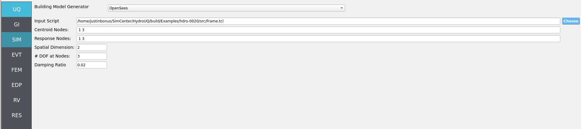
The structural model is as follows: a 2D, 3-DOF OpenSees portal frame in OpenSees, OpenSees.
Fig. 4.4.2.3.1 2D 3-DOF portal frame under stochastic wave loading (JONSWAP)
For the OpenSees generator the following model script, Frame.tcl , is used:
Click to expand the OpenSees input file used for this example
  1# Create ModelBuilder (with two-dimensions and 3 DOF/node)
  2
  3model basic -ndm 2 -ndf 3
  4
  5set width    360
  6set height   144
  7
  8node  1       0.0     0.0
  9node  2    $width     0.0
 10node  3       0.0 $height
 11node  4    $width $height
 12
 13fix   1     1    1    1
 14fix   2     1    1    1
 15
 16# Concrete ( Youngs Modulus, Yield Strength, and Compressive Strength)
 17pset fc 6.0
 18pset fy 60.0
 19pset E 30000.0
 20uniaxialMaterial Concrete01  1  -$fc  -0.004   -5.0     -0.014
 21uniaxialMaterial Concrete01  2  -5.0   -0.002   0.0     -0.006
 22
 23# STEEL
 24uniaxialMaterial Steel01  3  $fy $E 0.01
 25
 26set colWidth 15
 27set colDepth 24
 28set cover  1.5
 29set As    0.60;     # area of no. 7 bars
 30set y1 [expr $colDepth/2.0]
 31set z1 [expr $colWidth/2.0]
 32
 33section Fiber 1 {
 34
 35    # Create the concrete core fibers
 36    patch rect 1 10 1 [expr $cover-$y1] [expr $cover-$z1] [expr $y1-$cover] [expr $z1-$cover]
 37
 38    # Create the concrete cover fibers (top, bottom, left, right)
 39    patch rect 2 10 1  [expr -$y1] [expr $z1-$cover] $y1 $z1
 40    patch rect 2 10 1  [expr -$y1] [expr -$z1] $y1 [expr $cover-$z1]
 41    patch rect 2  2 1  [expr -$y1] [expr $cover-$z1] [expr $cover-$y1] [expr $z1-$cover]
 42    patch rect 2  2 1  [expr $y1-$cover] [expr $cover-$z1] $y1 [expr $z1-$cover]
 43
 44    # Create the reinforcing fibers (left, middle, right)
 45    layer straight 3 3 $As [expr $y1-$cover] [expr $z1-$cover] [expr $y1-$cover] [expr $cover-$z1]
 46    layer straight 3 2 $As 0.0 [expr $z1-$cover] 0.0 [expr $cover-$z1]
 47    layer straight 3 3 $As [expr $cover-$y1] [expr $z1-$cover] [expr $cover-$y1] [expr $cover-$z1]
 48
 49}
 50
 51
 52# Define column elements
 53# ----------------------
 54
 55# Geometry of column elements
 56#                tag
 57
 58geomTransf Corotational 1
 59
 60# Number of integration points along length of element
 61set np 5
 62
 63# Create the coulumns using Beam-column elements
 64#               e            tag ndI ndJ nsecs secID transfTag
 65set eleType dispBeamColumn
 66element $eleType  1   1   3   $np    1       1
 67element $eleType  2   2   4   $np    1       1
 68
 69# Define beam elment
 70# -----------------------------
 71
 72# Geometry of column elements
 73#                tag
 74geomTransf Linear 2
 75
 76# Create the beam element
 77#                          tag ndI ndJ     A       E    Iz   transfTag
 78element elasticBeamColumn   3   3   4    360    4030  8640    2
 79
 80# Define gravity loads
 81# --------------------
 82
 83# Set a parameter for the axial load
 84set P 180;                # 10% of axial capacity of columns
 85
 86# Create a Plain load pattern with a Linear TimeSeries
 87pattern Plain 1 "Linear" {
 88
 89        # Create nodal loads at nodes 3 & 4
 90	#    nd    FX          FY  MZ
 91	load  3   0.0  [expr -$P] 0.0
 92	load  4   0.0  [expr -$P] 0.0
 93}
 94
 95# ------------------------------
 96# Start of analysis generation
 97# ------------------------------
 98
 99# Create the system of equation, a sparse solver with partial pivoting
100system ProfileSPD
101
102# Create the constraint handler, the transformation method
103constraints Transformation
104
105# Create the DOF numberer, the reverse Cuthill-McKee algorithm
106numberer RCM
107
108# Create the convergence test, the norm of the residual with a tolerance of
109# 1e-12 and a max number of iterations of 10
110test NormDispIncr 1.0e-12  10 3
111
112# Create the solution algorithm, a Newton-Raphson algorithm
113algorithm Newton
114
115# Create the integration scheme, the LoadControl scheme using steps of 0.1
116integrator LoadControl 0.1
117
118# Create the analysis object
119analysis Static
120
121# ------------------------------
122# End of analysis generation
123# ------------------------------
124
125# perform the gravity load analysis, requires 10 steps to reach the load level
126analyze 10
127
128loadConst -time 0.0
129
130# ----------------------------------------------------
131# End of Model Generation & Initial Gravity Analysis
132# ----------------------------------------------------
133
134
135# ----------------------------------------------------
136# Start of additional modelling for dynamic loads
137# ----------------------------------------------------
138
139# Define nodal mass in terms of axial load on columns
140set g 386.4
141set m [expr $P/$g];       # expr command to evaluate an expression
142
143#    tag   MX   MY   RZ
144mass  3    $m   $m    0
145mass  4    $m   $m    0
Note
The first lines containing pset in an OpenSees tcl file will be read by the application when the file is selected. The application will autopopulate the random variables in the RV panel with these same variable names.
These variable names (fc, fy, E) are recognized in Frame.tcl due to use of the pset command instead of set. This is so that RV picks them up automatically. You can try adding new RV parameters in the same way.
Uncertain properties (treated as RVs; see Step 7):
fc: mean6, stdev0.06fy: mean60, stdev0.6E: mean30000, stdev300
4.4.2.4. Step 4: EVT
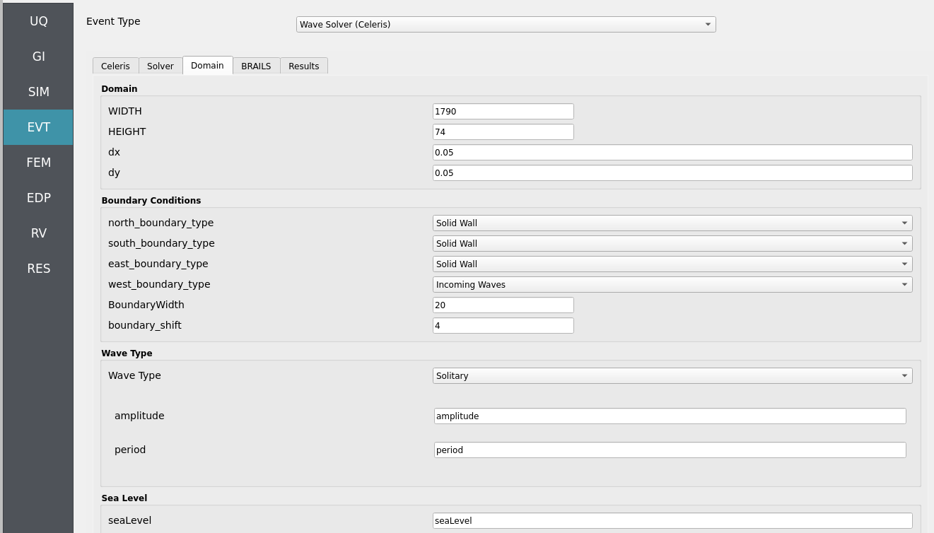
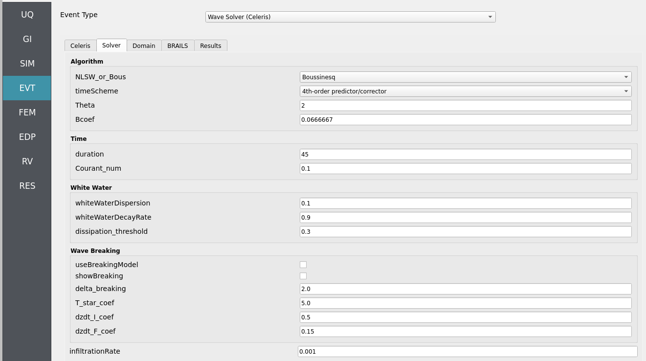
Load Generator: Celeris Event - Near-Real-Time Boussinesq Solver (scaled-down tsunami experiment replication by Winter 2019 and Mascarenas 2022).
Configuration outline:
Flume geometry: match the OSU LWF dimensions and bathymetry inserts used in Winter (2019) / Mascarenas (2022).
Wavemaker: piston-driven solitary wave; define nominal stroke/profile.
Instrumentation: place wave-gauges, velocimeters, and load-cells (virtual probes) at the experimental stations for comparison.
Hydrodynamic RVs: promote amplitude and period (solitary wave) and the quasi-static seaLevel offset to RVs (see Step 7).
Export: time histories (surface elevation, depth-averaged velocity, and forces/pressures) at probe and structure locations for load mapping.
To perform the manual workflow, load-in the following files to the Celeris tab:
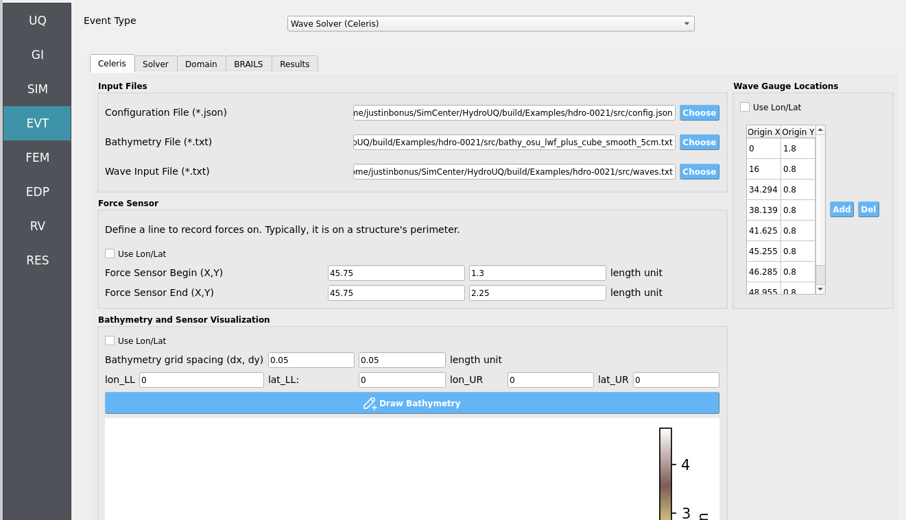
Double-check that the following parameters are set in the Solver and Domain tabs:
Note
We will not be using the BRAILS tab in this instance, as we are not concerned with modeling a full-scale, real-world rendition of these experiments and instead rely on the manually inputted files for experimental replication.
Advanced Exercise - Extrapolate to the Prototype Event
As an exercise for advanced users, try using the BRAILS tab to identify a suitable real-world location and building inventory that could represent the full-scale, prototype event. This involves searching for a coastal site with similar bathymetry and a structure matching the square footprint and approximate blockage ratio (0.28) used in the experiment. You must also ensure appropriate Froude similitude scaling of the incoming wave, and potentially surf similitude scaling of the bathymetry as well.
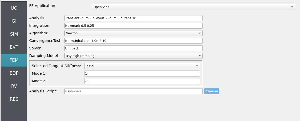
4.4.2.5. Step 5: FEM
Solver: OpenSees dynamic analysis. Check:
Integration step compatible with CelerisAi output interval.
Algorithm/convergence tolerances suitable for expected nonlinearity.
Damping model as needed (e.g., Rayleigh).
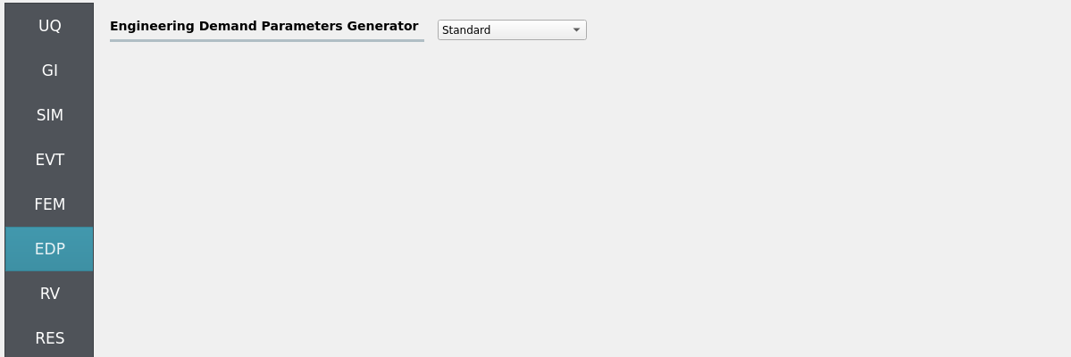
4.4.2.6. Step 6: EDP
Select Engineering Demand Parameters (EDPs) to summarize response:
Peak Floor Acceleration (PFA)
Root Mean Square Acceleration (RMSA)
Peak Floor Displacement (PFD)
Peak Interstory Drift (PID)
4.4.2.7. Step 7: RV
Define distributions for structural and hydrodynamic RVs:
Structural
fc: Normal (mean6, stdev0.06)fy: Normal (mean60, stdev0.6)E: Normal (mean30000, stdev300)
Hydrodynamic (solitary wave + mean level)
amplitude: Normal (mean0.5, stdev0.15)period: Normal (mean20, stdev4)seaLevel: Normal (mean2.0, stdev0.1)
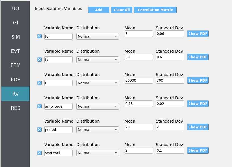
Warning
Ensure positivity of wave parameters (e.g., amplitude) if using Normal distributions—consider truncation or alternative distributions if needed.
4.4.3. Simulation
This workflow is intended for either local execution or remote execution to leverage near-real-time Celeris computation. Click RUN for local if you have a decently strong computer, or RUN at DesignSafe if you have a DesignSafe account and wish to use the Stampede3 supercomputer. When complete, the RES panel opens. Locally, the workflow will take from 20 to 60 minutes depending on your PC.
Warning
Keep recorder counts, export frequency, and sample size reasonable. Excessive export rates or too many recorders can dominate runtime and disk usage.
4.4.4. Analysis
Visualize time-series from event probes (e.g., wave-gauges, velocimeters, and load-sensors) by navigating to EVT / Wave Solver (Celeris) / Results. Then set the Run Type to Local for local workflows and choose the simulation you wish to inspect by setting Simulation Number between 1 and the number of samples you set in the UQ tab.
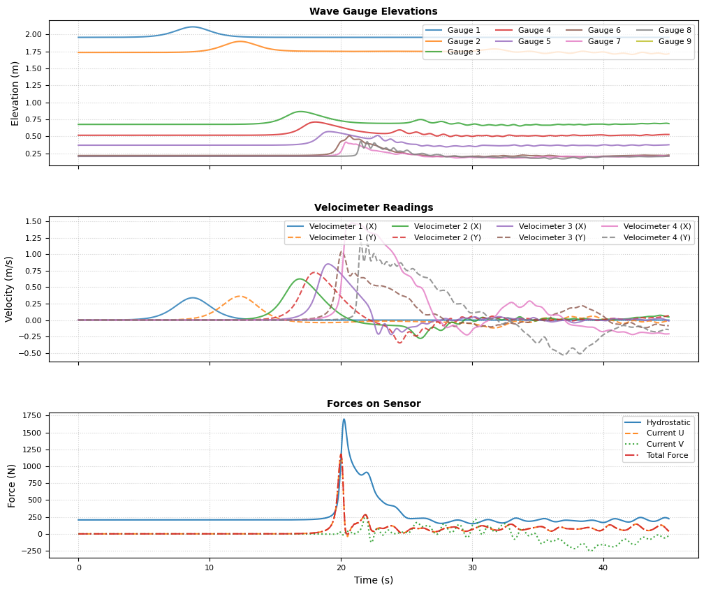
Wave-gauges & velocimeters: generally match experimental counterparts well at the instrumented locations.
Load-cells: simulated forces overpredict experiments. Reason: the solver is 2D depth-averaged, and the raised structural box was approximated as a square column embedded in the bathymetry—preventing underflow beneath the box, thus increasing hydrodynamic loads compared to the physical experiment where water could flow underneath.
Note
This HydroUQ example runs the Celeris configuration natively. Experimental results can be imported (optional) for side-by-side plots in the Analysis section for a comparative study, as in Bonus (2023). Acquire said data from: PRJ-2906.
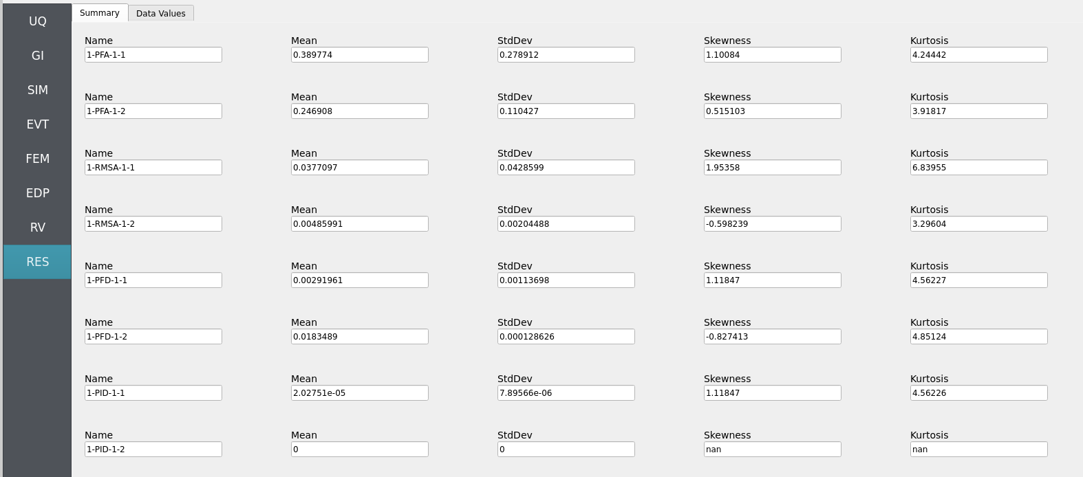
Returning to our primary HydroUQ workflow, which concerns uncertainty in structural response, we may now view the final results in the RES tab. Clicking Summary on the top-bar, a statistical summary of results is shown below:
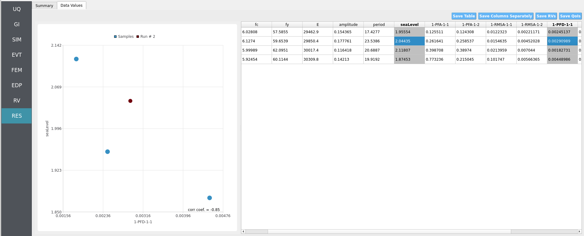
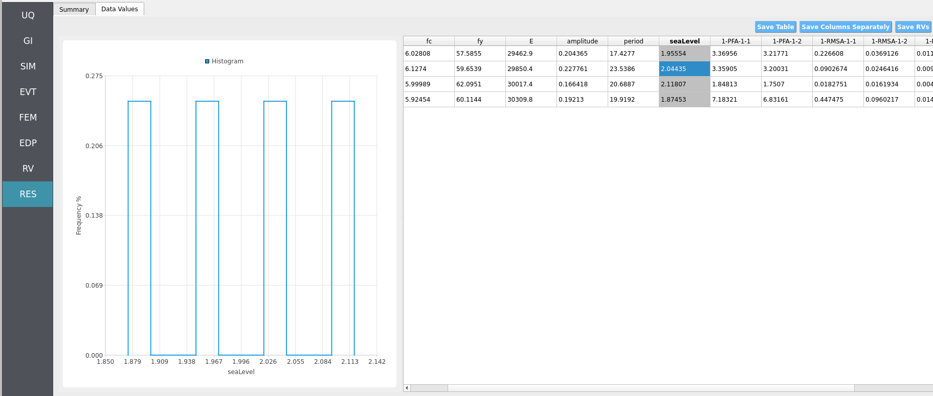
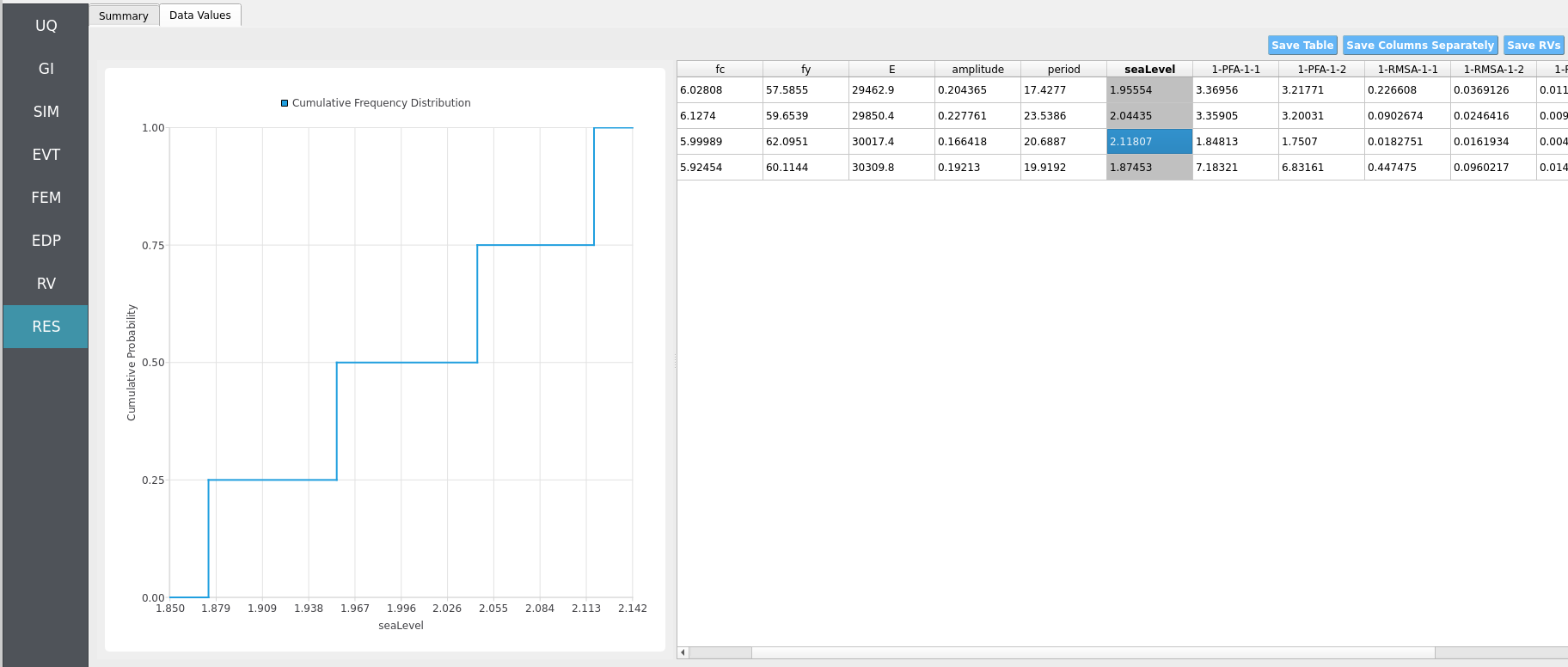
Clicking Data Values on the top-bar shows detailed histograms, cumulative distribution functions, and scatter plots relating the dependent and independent variables:
Note
In the Data Values tab, left- and right-click column headers to change plot axes; selecting a single column with both clicks displays frequency and CDF plots.
Note
Use consistent Froude similitude scaling when comparing numerical simulations, experiments, and full-scale scenarios. For cross-method comparisons, adopt identical structure footprints, friction models, probe placement, and other pertinent parameters to reduce bias.
For more advanced analysis, export results as a CSV file by clicking Save Table on the upper-right of the application window. This will save the independent and dependent variable data. I.e., the Random Variables you defined and the Engineering Demand Parameters determined from the structural response per each simulation.
To save your simulation configuration with results included, click File / Save As and specify a location for the HydroUQ JSON input file to be recorded to. You may then reload the file at a later time by clicking File / Open. You may also send it to others by email or place it in an online repository for research reproducibility. This example’s input file is viewable at Reproducibility.
To directly share your simulation job and results in HydroUQ with other DesignSafe users, click GET from DesignSafe. Then, navigate to the row with your job and right-click it. Select Share Job. You may then enter the DesignSafe username or usernames (comma-separated) to share with.
Important
Sharing a job requires that the job was initially ran with an Archive System ID (listed in the GET from DesignSafe table’s columns) that is not designsafe.storage.default. Any other Archive System ID allows for sharing with DesignSafe members on the associated project. See Jobs for more details.
4.4.5. Conclusions
We have successfully replicated experiments in OSU’s Large Wave Flume using Celeris. Load-cell overpredictions arise because a 2D depth-averaged model approximated a raised structural box as a solid square column, blocking underflow and elevating forces. Because the loads come from a flume-scale scenario, mapping them directly to a full-scale structural model can underpredict (or misrepresent) EDPs. This highlights the need to scale the structure or scale the forces using similitude laws, which is left as an exercise for the reader.
4.4.6. References
Winter, A. (2019). “Effects of Flow Shielding and Channeling on Tsunami-Induced Loading of Coastal Structures.” PhD thesis. University of Washington, Seattle.
Mascarenas, Dakota. (2022). “Quantification of Wave-Driven Debris Impact on a Raised Structure in a Large Wave Flume.” Masters thesis. University of Washington, Seattle.
Bonus, Justin (2023). “Evaluation of Fluid-Driven Debris Impacts in a High-Performance Multi-GPU Material Point Method.” PhD thesis. University of Washington, Seattle.
4.4.7. Reproducibility
Random seed(s):
1(set in UQ)Model file:
Frame.tclApp version: HydroUQ v4.2.0
Wave solver: Celeris (as provided in NHERI-SimCenter/SimCenterBackendApplications)
System: Local Mac, Linux, and Windows, as well as TACC HPC clusters such as Stampede3.
Input: The HydroUQ input file is as follows: input.json , is used:
Click to expand the HydroUQ input file used for this example
1{
2 "Applications": {
3 "EDP": {
4 "Application": "StandardEDP",
5 "ApplicationData": {
6 }
7 },
8 "Events": [
9 {
10 "Application": "Celeris",
11 "ApplicationData": {
12 },
13 "EventClassification": "Hydro"
14 }
15 ],
16 "Modeling": {
17 "Application": "OpenSeesInput",
18 "ApplicationData": {
19 "fileName": "Frame.tcl",
20 "filePath": "{Current_Dir}/."
21 }
22 },
23 "Simulation": {
24 "Application": "OpenSees-Simulation",
25 "ApplicationData": {
26 }
27 },
28 "UQ": {
29 "Application": "Dakota-UQ",
30 "ApplicationData": {
31 }
32 }
33 },
34 "DefaultValues": {
35 "driverFile": "driver",
36 "edpFiles": [
37 "EDP.json"
38 ],
39 "filenameAIM": "AIM.json",
40 "filenameDL": "BIM.json",
41 "filenameEDP": "EDP.json",
42 "filenameEVENT": "EVENT.json",
43 "filenameSAM": "SAM.json",
44 "filenameSIM": "SIM.json",
45 "rvFiles": [
46 "AIM.json",
47 "SAM.json",
48 "EVENT.json",
49 "SIM.json"
50 ],
51 "workflowInput": "scInput.json",
52 "workflowOutput": "EDP.json"
53 },
54 "EDP": {
55 "type": "StandardEDP"
56 },
57 "Events": [
58 {
59 "Application": "Celeris",
60 "EventClassification": "Hydro",
61 "type": "Celeris",
62 "bathymetryFile": "bathy_osu_lwf_plus_cube_smooth_5cm.txt",
63 "bathymetryFilePath": "{Current_Dir}/.",
64 "config": {
65 "Bcoef": 0.06666667,
66 "Bcoef_g": 0.6540000327,
67 "BoundaryWidth": 20,
68 "CB_label_height": 10,
69 "CB_show": 1,
70 "CB_width": 805,
71 "CB_width_uv": 0.9,
72 "CB_xbuffer": 8,
73 "CB_xbuffer_uv": 0.01,
74 "CB_xstart": 45,
75 "CB_xstart_uv": 0.05,
76 "CB_ystart": 30,
77 "Courant_num": 0.1,
78 "DispatchX": 55,
79 "DispatchY": 28,
80 "GMapImageHeight": 512,
81 "GMapImageWidth": 512,
82 "GMoffsetX": 0,
83 "GMoffsetY": 0,
84 "GMscaleX": 1,
85 "GMscaleY": 1,
86 "GoogleMapOverlay": 0,
87 "HEIGHT": 74,
88 "IsGoogleMapLoaded": 0,
89 "NLSW_or_Bous": 1,
90 "NumberOfTimeSeries": 8,
91 "PI": 3.141592653589793,
92 "TWO_THETA": 4,
93 "Theta": 2,
94 "ThreadX": 16,
95 "ThreadY": 16,
96 "WIDTH": 1790,
97 "WaveType": 3,
98 "add_Disturbance": -1,
99 "amplitude": "RV.amplitude",
100 "base_depth": "RV.seaLevel",
101 "boundary_epsilon": 5.6553838196257955e-09,
102 "boundary_g": 9.81,
103 "boundary_nx": 872,
104 "boundary_ny": 436,
105 "boundary_shift": 4,
106 "canvas_height_ratio": 1,
107 "canvas_width_ratio": 1,
108 "changeAmplitude": 0.07520228600000001,
109 "changeRadius": 2.5,
110 "changeType": 1,
111 "changeXTimeSeries": 0,
112 "changeYTimeSeries": 0,
113 "changethisTimeSeries": 5,
114 "chartDataUpdate": 0,
115 "clearConc": 0,
116 "click_update": -1,
117 "colorMap_choice": 0,
118 "colorVal_max": 1,
119 "colorVal_min": -1,
120 "countTimeSeries": 9079,
121 "direction": 0,
122 "dissipation_threshold": 0.3,
123 "disturbanceCrestamp": 0.6,
124 "disturbanceDip": 0,
125 "disturbanceDir": 0,
126 "disturbanceLength": 0,
127 "disturbanceRake": 0,
128 "disturbanceType": 1,
129 "disturbanceWidth": 0,
130 "disturbanceXpos": 3,
131 "disturbanceYpos": 0,
132 "dt": 0.0036817133736190564,
133 "duration": 45.0,
134 "durationTimeSeries": 0,
135 "dx": 0.05,
136 "dy": 0.05,
137 "east_boundary_type": 0,
138 "elapsedTime": 204.542,
139 "elapsedTime_update": 45.224,
140 "exampleDirs": [
141 "./examples/Ventura/",
142 "./examples/Santa_Cruz/",
143 "./examples/Santa_Cruz_tsunami/",
144 "./examples/Barry_Arm/",
145 "./examples/Crescent_City/",
146 "./examples/DuckFRF_NC/",
147 "./examples/Greenland/",
148 "./examples/Half_Moon_Bay/",
149 "./examples/Hania_Greece/",
150 "./examples/Miami_Beach_FL/",
151 "./examples/Miami_FL/",
152 "./examples/Newport_OR/",
153 "./examples/POLALB/",
154 "./examples/SantaBarbara/",
155 "./examples/Taan_fjord/",
156 "./examples/OSU_WaveBasin/",
157 "./examples/SF_Bay_tides/"
158 ],
159 "force_sensor_begin": [45.75, 1.30],
160 "force_sensor_end": [45.75, 2.25],
161 "forward": 1,
162 "friction": 0.001,
163 "full_screen": 0,
164 "g": 9.80665,
165 "g_over_dx": 196.2,
166 "g_over_dy": 196.2,
167 "half_g": 4.905,
168 "html_update": -1,
169 "isManning": 0,
170 "lat_LL": 0,
171 "lat_UR": 0,
172 "locationOfTimeSeries": [
173 {
174 "name": "WaveMaker",
175 "xts": 0,
176 "yts": 1.8
177 },
178 {
179 "name": "WG1",
180 "xts": 16,
181 "yts": 0.8
182 },
183 {
184 "name": "WG2",
185 "xts": 34.294,
186 "yts": 0.8
187 },
188 {
189 "name": "WG3",
190 "xts": 38.139,
191 "yts": 0.8
192 },
193 {
194 "name": "USWG1",
195 "xts": 41.625,
196 "yts": 0.8
197 },
198 {
199 "name": "USWG2",
200 "xts": 45.255,
201 "yts": 0.8
202 },
203 {
204 "name": "USWG3",
205 "xts": 46.285,
206 "yts": 0.8
207 },
208 {
209 "name": "USWG4",
210 "xts": 48.955,
211 "yts": 0.8
212 }
213 ],
214 "lon_LL": 0,
215 "lon_UR": 0,
216 "maxNumberOfTimeSeries": 16,
217 "maxdurationTimeSeries": 30,
218 "mouse_current_canvas_indX": 219,
219 "mouse_current_canvas_indY": 4,
220 "mouse_current_canvas_positionX": 0,
221 "mouse_current_canvas_positionY": 0,
222 "n_time_steps_means": 47290,
223 "n_time_steps_waveheight": 47290,
224 "n_write_interval": null,
225 "n_writes": null,
226 "north_boundary_type": 0,
227 "numberOfWaves": 2961,
228 "one_over_d2x": 400,
229 "one_over_d2y": 400,
230 "one_over_d3x": 8000,
231 "one_over_d3y": 8000,
232 "one_over_dx": 20,
233 "one_over_dxdy": 400,
234 "one_over_dy": 20,
235 "period": "RV.period",
236 "pred_or_corrector": 2,
237 "rand_phase": 0,
238 "reflect_x": 1740,
239 "reflect_y": 868,
240 "render_step": 4,
241 "rotationAngle_xy": 0,
242 "run_example": 0,
243 "save_baseline": 0,
244 "seaLevel": "RV.seaLevel",
245 "sedC1_criticalshields": 0.045,
246 "sedC1_d50": 0.2,
247 "sedC1_denrat": 2.65,
248 "sedC1_erosion": 0.0002746401358265295,
249 "sedC1_fallvel": 0.14690813456034352,
250 "sedC1_n": 0.4,
251 "sedC1_psi": 5e-05,
252 "sedC1_shields": 308.8993914681988,
253 "shift_x": 0,
254 "shift_y": 0,
255 "ship_c1a": 0.005483113556160754,
256 "ship_c1b": 0.04934802200544678,
257 "ship_c2": 0.021932454224643013,
258 "ship_c3a": 0.005483113556160754,
259 "ship_c3b": 0.04934802200544678,
260 "ship_draft": 2,
261 "ship_heading": 0,
262 "ship_length": 30,
263 "ship_posx": -100,
264 "ship_posy": 450,
265 "ship_width": 10,
266 "useBreakingModel": 0,
267 "showBreaking": 0,
268 "significant_wave_height": 1,
269 "simPause": -1,
270 "south_boundary_type": 0,
271 "surfaceToChange": 1,
272 "surfaceToPlot": 0,
273 "timeScheme": 2,
274 "tooltipVal_Hs": 0.17761249840259552,
275 "tooltipVal_bottom": -0.6820381879806519,
276 "tooltipVal_eta": 0.045800093561410904,
277 "tooltipVal_friction": 0.0010000000474974513,
278 "tridiag_solve": 2,
279 "updateTimeSeriesTx": 0,
280 "useSedTransModel": 0,
281 "viewType": 1,
282 "west_boundary_type": 2,
283 "whiteWaterDecayRate": 0.9,
284 "write_dt": null,
285 "xClick": 0,
286 "yClick": 0
287 },
288 "configFile": "config.json",
289 "configFilePath": "{Current_Dir}/.",
290 "waveFile": "waves.txt",
291 "waveFilePath": "{Current_Dir}/."
292 }
293 ],
294 "GeneralInformation": {
295 "NumberOfStories": 1,
296 "PlanArea": 129600,
297 "StructureType": "RM1",
298 "YearBuilt": 1990,
299 "depth": 360,
300 "height": 576,
301 "location": {
302 "latitude": 37.8715,
303 "longitude": -122.273
304 },
305 "name": "",
306 "planArea": 129600,
307 "stories": 1,
308 "units": {
309 "force": "kips",
310 "length": "in",
311 "temperature": "C",
312 "time": "sec"
313 },
314 "width": 360
315 },
316 "Modeling": {
317 "centroidNodes": [
318 1,
319 3
320 ],
321 "dampingRatio": 0.02,
322 "ndf": 3,
323 "ndm": 2,
324 "randomVar": [
325 {
326 "name": "fc",
327 "value": "RV.fc"
328 },
329 {
330 "name": "fy",
331 "value": "RV.fy"
332 },
333 {
334 "name": "E",
335 "value": "RV.E"
336 }
337 ],
338 "responseNodes": [
339 1,
340 3
341 ],
342 "type": "OpenSeesInput"
343 },
344 "Simulation": {
345 "Application": "OpenSees-Simulation",
346 "algorithm": "Newton",
347 "analysis": "Transient -numSubLevels 2 -numSubSteps 10",
348 "convergenceTest": "NormUnbalance 1.0e-2 10",
349 "dampingModel": "Rayleigh Damping",
350 "firstMode": 1,
351 "integration": "Newmark 0.5 0.25",
352 "modalRayleighTangentRatio": 0,
353 "numModesModal": -1,
354 "rayleighTangent": "Initial",
355 "secondMode": -1,
356 "solver": "Umfpack"
357 },
358 "UQ": {
359 "parallelExecution": false,
360 "samplingMethodData": {
361 "method": "LHS",
362 "samples": 4,
363 "seed": 1
364 },
365 "saveWorkDir": true,
366 "uqType": "Forward Propagation"
367 },
368 "correlationMatrix": [
369 1,
370 0,
371 0,
372 0,
373 0,
374 0,
375 0,
376 1,
377 0,
378 0,
379 0,
380 0,
381 0,
382 0,
383 1,
384 0,
385 0,
386 0,
387 0,
388 0,
389 0,
390 1,
391 0,
392 0,
393 0,
394 0,
395 0,
396 0,
397 1,
398 0,
399 0,
400 0,
401 0,
402 0,
403 0,
404 1
405 ],
406 "localAppDir": "/home/justinbonus/SimCenter/HydroUQ/build",
407 "randomVariables": [
408 {
409 "distribution": "Normal",
410 "inputType": "Parameters",
411 "mean": 6,
412 "name": "fc",
413 "refCount": 1,
414 "stdDev": 0.06,
415 "value": "RV.fc",
416 "variableClass": "Uncertain"
417 },
418 {
419 "distribution": "Normal",
420 "inputType": "Parameters",
421 "mean": 60,
422 "name": "fy",
423 "refCount": 1,
424 "stdDev": 0.6,
425 "value": "RV.fy",
426 "variableClass": "Uncertain"
427 },
428 {
429 "distribution": "Normal",
430 "inputType": "Parameters",
431 "mean": 30000,
432 "name": "E",
433 "refCount": 1,
434 "stdDev": 300,
435 "value": "RV.E",
436 "variableClass": "Uncertain"
437 },
438 {
439 "distribution": "Normal",
440 "inputType": "Parameters",
441 "mean": 0.15,
442 "name": "amplitude",
443 "refCount": 0,
444 "stdDev": 0.02,
445 "value": "RV.amplitude",
446 "variableClass": "Uncertain"
447 },
448 {
449 "distribution": "Normal",
450 "inputType": "Parameters",
451 "mean": 20,
452 "name": "period",
453 "refCount": 0,
454 "stdDev": 2,
455 "value": "RV.period",
456 "variableClass": "Uncertain"
457 },
458 {
459 "distribution": "Normal",
460 "inputType": "Parameters",
461 "mean": 2,
462 "name": "seaLevel",
463 "refCount": 0,
464 "stdDev": 0.1,
465 "value": "RV.seaLevel",
466 "variableClass": "Uncertain"
467 }
468 ],
469 "remoteAppDir": "/home/justinbonus/SimCenter/HydroUQ/build",
470 "resultType": "SimCenterUQResultsSampling",
471 "runType": "runningLocal",
472 "spreadsheet": {
473 "data": [
474 1,
475 6.028075539,
476 57.58553221,
477 29462.85806,
478 0.2043653771,
479 17.42765996,
480 1.955543862,
481 3.36956,
482 3.21771,
483 0.226608,
484 0.0369126,
485 0.0114226,
486 0.0183792,
487 7.93233e-05,
488 0,
489 2,
490 6.127403326,
491 59.65390904,
492 29850.41289,
493 0.2277606611,
494 23.53859216,
495 2.044351917,
496 3.35905,
497 3.20031,
498 0.0902674,
499 0.0246416,
500 0.00969684,
501 0.0181782,
502 6.73391e-05,
503 0,
504 3,
505 5.99989415,
506 62.09509192,
507 30017.36909,
508 0.1664177408,
509 20.68867725,
510 2.118068995,
511 1.84813,
512 1.7507,
513 0.0182751,
514 0.0161934,
515 0.00484152,
516 0.0183701,
517 3.36217e-05,
518 0,
519 4,
520 5.924539779,
521 60.11436404,
522 30309.83223,
523 0.1921301395,
524 19.91918823,
525 1.874532636,
526 7.18321,
527 6.83161,
528 0.447475,
529 0.0960217,
530 0.0146628,
531 0.0185367,
532 0.000101825,
533 0
534 ],
535 "headings": [
536 "Run #",
537 "fc",
538 "fy",
539 "E",
540 "amplitude",
541 "period",
542 "seaLevel",
543 "1-PFA-1-1",
544 "1-PFA-1-2",
545 "1-RMSA-1-1",
546 "1-RMSA-1-2",
547 "1-PFD-1-1",
548 "1-PFD-1-2",
549 "1-PID-1-1",
550 "1-PID-1-2",
551 ""
552 ],
553 "isSurrogate": false,
554 "nrv": 6,
555 "numCol": 15,
556 "numRow": 4
557 },
558 "summary": [
559 {
560 "kurtosis": 5.614692499053245,
561 "mean": 3.9399875,
562 "name": "1-PFA-1-1",
563 "skewness": 1.3875429685905685,
564 "stdDev": 2.2772231552540037
565 },
566 {
567 "kurtosis": 5.591685203027151,
568 "mean": 3.7500825000000004,
569 "name": "1-PFA-1-2",
570 "skewness": 1.373905833853955,
571 "stdDev": 2.1663342613021817
572 },
573 {
574 "kurtosis": 2.971158918787393,
575 "mean": 0.195656375,
576 "name": "1-RMSA-1-1",
577 "skewness": 0.915894925818679,
578 "stdDev": 0.18880463956093832
579 },
580 {
581 "kurtosis": 5.8853965585463985,
582 "mean": 0.043442325000000004,
583 "name": "1-RMSA-1-2",
584 "skewness": 1.6791609968413177,
585 "stdDev": 0.03607029783699002
586 },
587 {
588 "kurtosis": 3.8412299933476675,
589 "mean": 0.010155939999999999,
590 "name": "1-PFD-1-1",
591 "skewness": -0.5486350725435686,
592 "stdDev": 0.00409756217612375
593 },
594 {
595 "kurtosis": 4.549094901699577,
596 "mean": 0.01836605,
597 "name": "1-PFD-1-2",
598 "skewness": -0.34957985444781725,
599 "stdDev": 0.00014674055335864089
600 },
601 {
602 "kurtosis": 3.8412471088843487,
603 "mean": 7.052727500000001e-05,
604 "name": "1-PID-1-1",
605 "skewness": -0.5486176664419157,
606 "stdDev": 2.8455248911741514e-05
607 },
608 {
609 "kurtosis": null,
610 "mean": 0,
611 "name": "1-PID-1-2",
612 "skewness": null,
613 "stdDev": 0
614 }
615 ],
616 "workingDir": "/home/justinbonus/Documents/HydroUQ/LocalWorkDir"
617}