4.8. Debris in Steady-State Flow - Digital Flume (UW WASIRF) - MPM
Problem files |
4.8.1. Outline
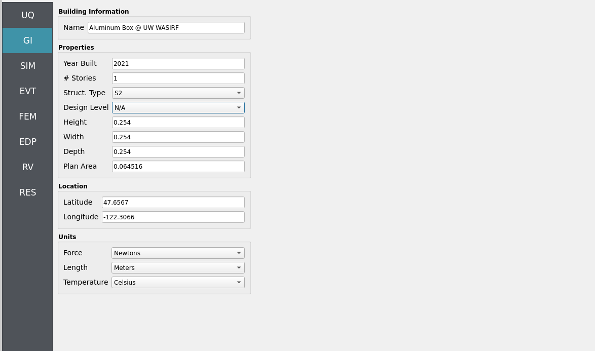
Fig. 4.8.1.1 GUI for the University of Washington’s Wind and Sea Interaction Facility (UW WASIRF).
This example examines steady-flow debris impacts on a raised structure by constructing a Material Point Method (MPM, [Bonus2023Dissertation] and [Bonus2025ClaymoreUW]) digital flume of the UW Washington Air–Sea Interaction Research Facility (WASIRF) debris tests (Lewis 2021–2023, [Lewis2023] and [Lewis2023Dissertation]). WASIRF provides a 1:4 geometric down-scale of OSU LWF debris-load experiments and simulations, see Multiple Debris Impacts on a Raised Structure - Digital Flume (OSU LWF) - MPM, so approximately 1:40 of a prototype tsunami event, using pump-driven, near-steady hydrodynamics and optional wave or wind forcing. Here we focus on the steady water inflow cases without wind effects. We will replicate the pump-driven inflow / outflow of the flume by virtually extending it and applying a velocity boundary condition to the incoming fluid, but it should be noted with some effort that more traditional pressure boundary inflow / outflow conditions can be simulated. Key aspects of these tests are:
Hydrodynamics: pump-driven flow achieving a target depth–velocity pair from experiments; inflow/outflow emulated numerically via upstream/downstream velocity buffer zones (mass conserved).
Structure: the raised aluminum box (1:4 of the “orange box” from Multiple Debris Impacts on a Raised Structure - Digital Flume (OSU LWF) - MPM) modeled as a rigid, separable boundary with numerical load-cells (node-wise force integration on the front face).
Debris: HDPE prisms (vehicle or boat surrogates) placed ~0.8 m upstream; spacing chosen to replicate the rate at which the experimentalists tended to drop debris into the flow during tests.
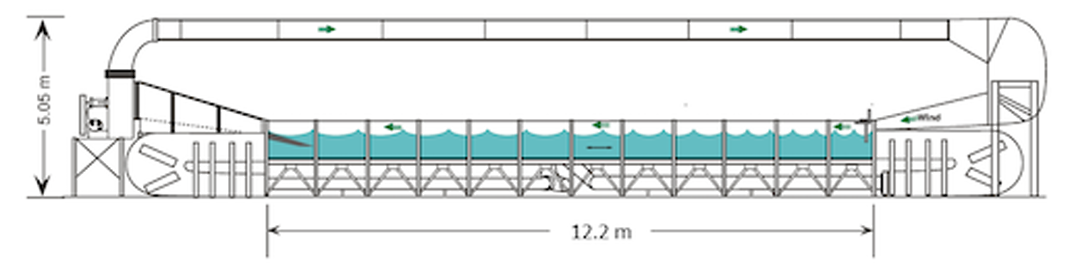
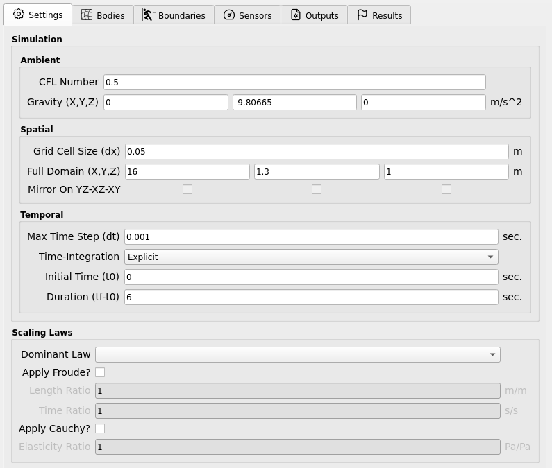
Fig. 4.8.1.2 Schematic for the University of Washington’s Wind and Sea Interaction Facility (UW WASIRF).
Our HydroUQ workflow in this example will study structural response of the aluminum box to fluid-debris loading. However, we note that underlying experiments had the goal of studying comprehensive fluid-debris phenomena in tandem with structural loading. For more advanced analysis for motivated readers, we may recommend tracking the below Quantities of interest (QoIs) and non-dimensional metrics in the context of hydrodynamic and debris UQ:
Incoming Froude number at the last upstream station before impact: \(Fr = U_f / \sqrt{g\,h_f}\), with \(U_f\) and \(h_f\) measured from ADV or wave-gauge proxies in the simulation.
Force coefficient and impulse at the wall: \(C_F = F / (\rho\,U_f^2\,A)\), \(J^* = \left(\int F(t)\,dt\right) / (\rho\,U_f^2\,A\,T_c)\), where \(A\) is the box projected area and \(T_c\) a characteristic passage time (for example, debris-front width \(L_f/U_f\)).
Plateau-to-peak load ratio \(R_{PP} = F_{\text{plateau}}/F_{\text{peak}}\) to quantify buffering and damming under steady inflow.
Front porosity \(\Phi\) and blockage ratio \(\beta = A_{\text{blocked}}/A_{\text{flow}}\) of the debris pack, governing water leakage and momentum transfer.
Debris kinematics: center-of-mass speed ratio \(U_d/U_f\), breakup length scale \(L_b\), and re-organization patterns at the structure.
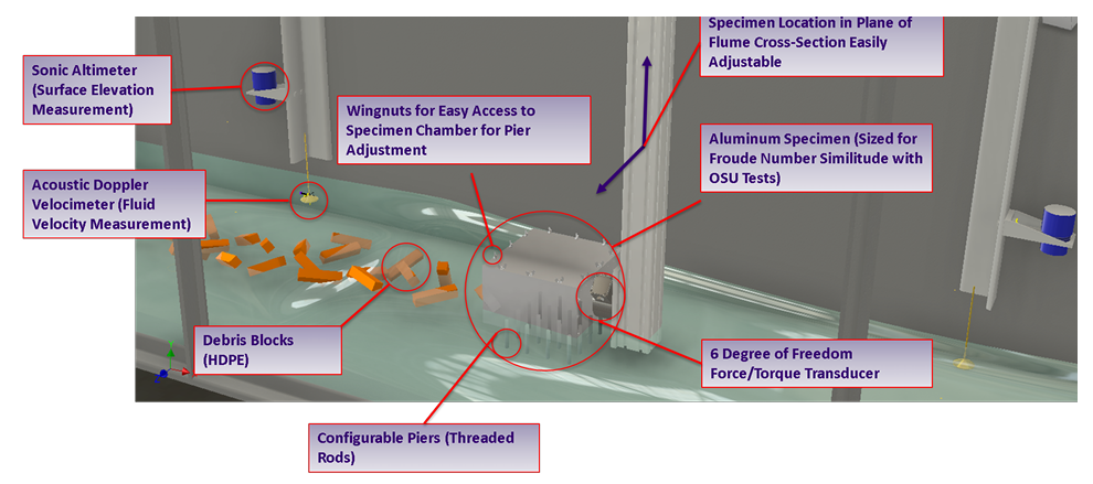
Fig. 4.8.1.3 Digital rendition of the University of Washington’s Wind and Sea Interaction Facility (UW WASIRF) to illustrate sensor placement and debris relative to the raised structural box.
4.8.2. Set-Up
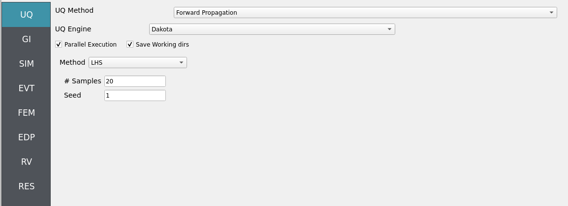
4.8.2.1. Step 1: UQ
Configure Forward sampling to explore structural/material uncertainty under a fixed hydrodynamic signal.
Engine: Dakota
Forward Propagation: Sampling method (e.g., LHS) with
samples(e.g.,20) and a reproducibleseed(e.g.,1).
4.8.2.2. Step 2: GI
Set General Information and Units consistent with experiments (length, time, density, gravity). Record project metadata.
Structure name:
Aluminum Box @ UW WASIRFUnits: choose a consistent set (e.g., N-m-s or kips-in-s)
Note
Keep GI, SIM, EVT, and FEM units consistent. Match MPM’s length/time scales and OpenSees integration settings (e.g., time step). Verify any force/unit conversions used during load mapping.
4.8.2.3. Step 3: SIM
The structural model is as follows: a single-story Multi-Degree-of-Freedom system (MDOF, see Multiple Degrees of Freedom (MDOF)) which we vertically invert to replicate the hanging, raised structural box in the UW WASIRF tests.
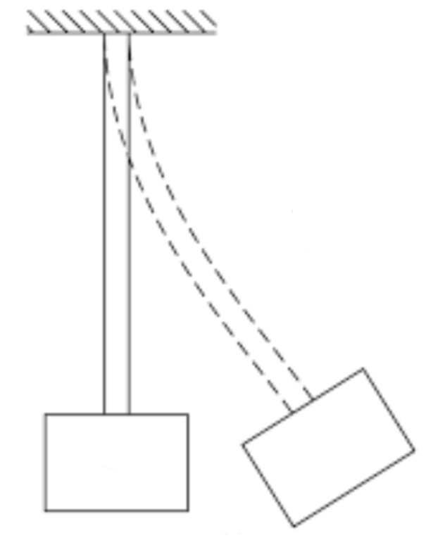
Fig. 4.8.2.3.1 Schematic of a single-story MDOF structure representing a structural box undergoing deflection from MPM derived hydrodynamic loading.
Note
The structure will be represented initially as a rigid boundary in MPM to recover local hydrodynamic forces at grid nodes for direct comparison with load-cell data. Structural dynamic response is added later by mapping these loads onto an OpenSees model defined here in the SIM panel with analysis options set in the FEM panel.
Uncertain structural properties (treated as RVs; see Step 7):
w: Weight. Mean144, stdev12
Bind parameters via setting alphabetic characters in the variable input boxes (e.g., w) so the RV panel recognizes and manages them automatically.
While not necessary to have, we show the template OpenSees model for your reference. The script generated in the backend by the MDOF module resembles the following, MDOF.tcl:
Click to expand the OpenSees input file used for this example
 1model BasicBuilder -ndm 3 -ndf 6
 2pset w 144.0
 3node 2 0 0 576 -mass $w $w  0.0  0.0  0.0  0.0
 4fix 2 0 0 1 1 1 0
 5node 1 0 0 0
 6fix 1 1 1 1 1 1 1
 7uniaxialMaterial Steel01 1 1e+06 100 0.1
 8uniaxialMaterial Steel01 2 1e+06 100 0.1
 9uniaxialMaterial Elastic 3 1e+10
10element zeroLength 1 1 2 -mat 1 2 3 -dir 1 2 6 -doRayleigh
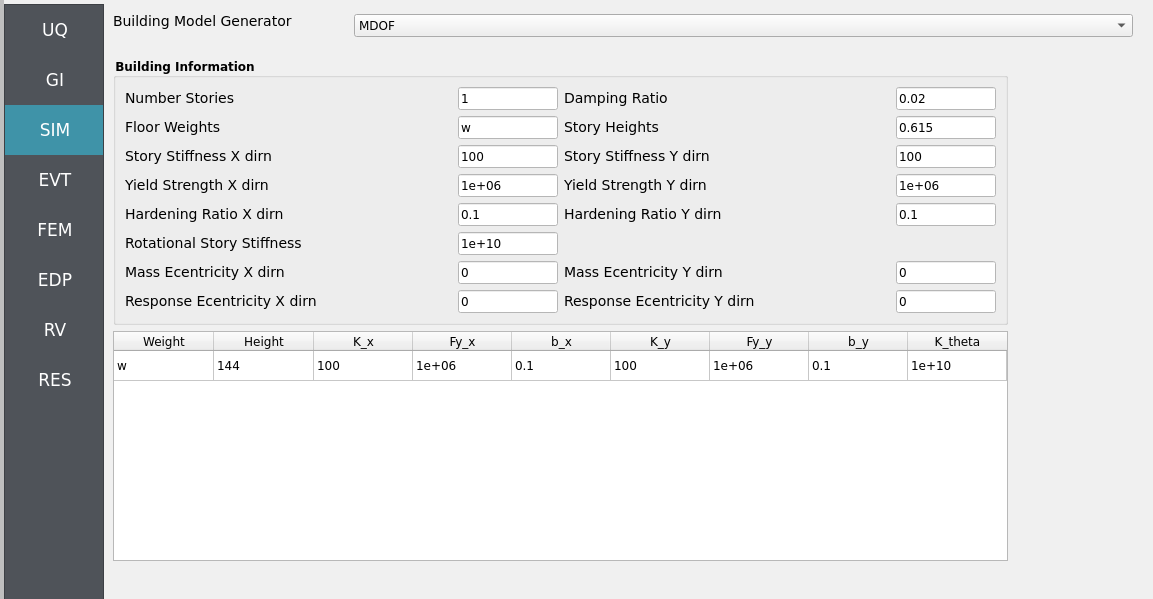
4.8.2.4. Step 4: EVT
In this walk-through we will give a detailed step-by-step configuration of the MPM EVT module.
Settings
Open Settings. Here we set the simulation time, the time step, and the grid resolution, among other pre-simulation decisions.
Bodies
Geometry
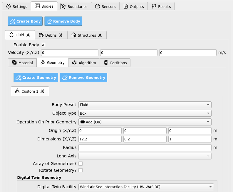
Fluid geometry
Open Bodies / Fluid / Geometry. Here we set the geometry of the flume’s fluid. Note that it is simply a rectangular prism which extends beyond the physical flume due to our velocity buffering approach for inflow / outflow used in this example.
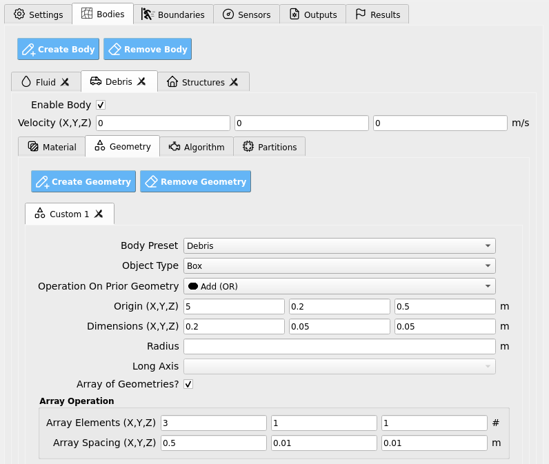
Debris geometry:
Open Bodies / Debris / Geometry. Here we set the debris properties, such as the number of debris, the size of the debris, and the spacing between the debris. Rotation is another option, though not used in this example. We’ve elected to use an 3 x 1 grid of debris (longitudinal axis parallel to long-axis of the flume).
Material
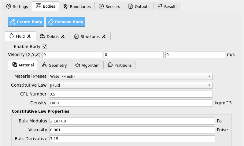
Fluid material:
Open Bodies / Fluid / Material. Here we set the material properties of the fluid. You may choose to use a realistic bulk modulus value of 2.1 GPa for the water, or you may soften it to 0.21 GPa to accelerate the simulation and reduce numerical stiffness with fairly minimal changes in our final results.
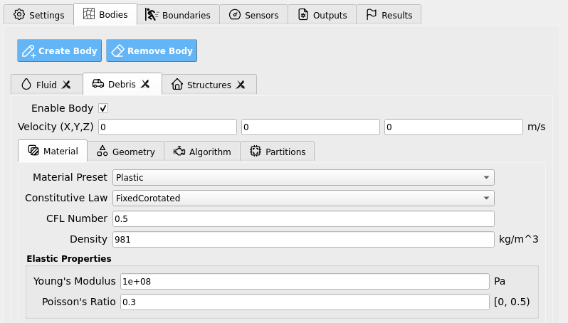
Debris material:
Moving onto the creation of an ordered debris array, we set the debris properties in the Bodies / Debris / Material tab. We will assume debris are made of HDPE plastic, as in experiments by Lewis 2023 [Lewis2023], Mascarenas 2022 [Mascarenas2022], and Shekhar et al. 2020 [Shekhar2020], and set properties accordingly.
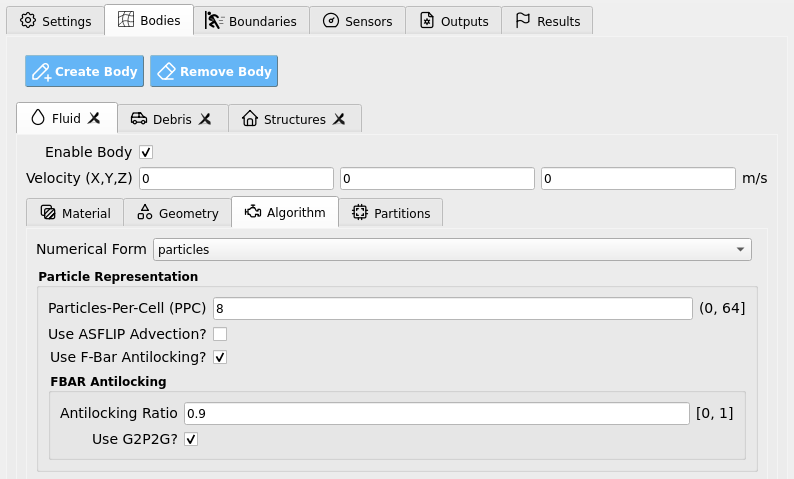
Algorithm
Open Bodies / Fluid / Algorithm. Here we set the algorithm parameters for the simulation. This is an advanced feature of the MPM module, it is best not to alter it too much. We choose to apply F-Bar antilocking to aid in the pressure field’s accuracy on the fluid. The associated toggle must be checked, and the antilocking ratio set to 0.9, loosely. For full bulk modulus water, you may need to increase this value to alleviate numerical stiffness.
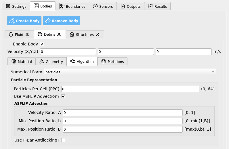
In Bodies / Debris / Algorithm we set debris for compatibility with the fluid as follows: ASFLIP is turned on and F-Bar antilocking is turned off. We keep ASFLIP tuning values at their default of zero as we do not need advanced behavior in this example.
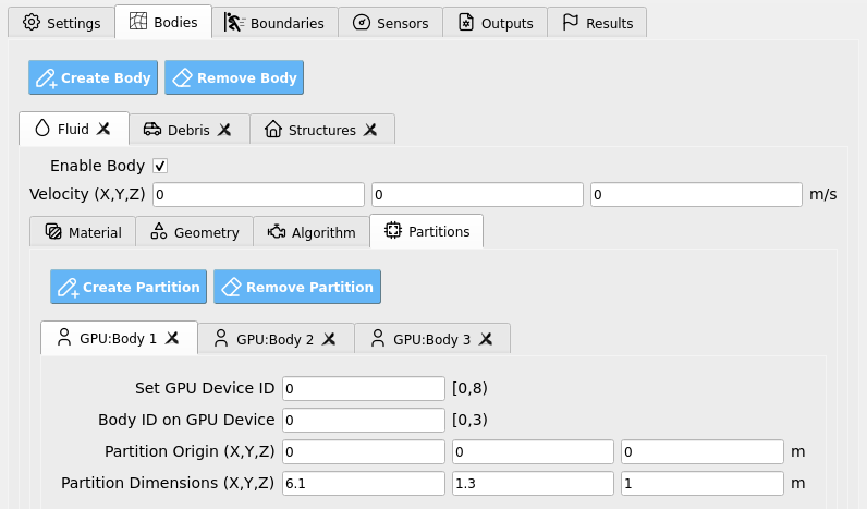
Partitions:
Open Bodies / Fluid / Partitions. This is an advanced feature of the MPM module which allows us to partition material bodies across hardware devices to optimize simulations. These may be kept as their default values, which have already been set for compatibility on the remote HPC system.
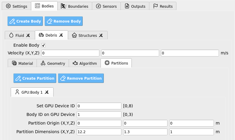
Next, Bodies / Debris / Partitions defines a partition where the debris may exist in our flume domain and defines the hardware device (i.e., GPU) that they will be simulated on. Keep this as the default unless you are an advanced user.
Structure:
Finally, open Bodies / Structures. Uncheck the box that enables this body. We will not model the structure as a deformable MPM material body in this example, instead, we will approximate it as a rigid MPM boundary a few steps from now. After the MPM simulation we will map loads from the boundary to an OpenSees structure for structural analysis, see Steps 3 and 5 for configuration.
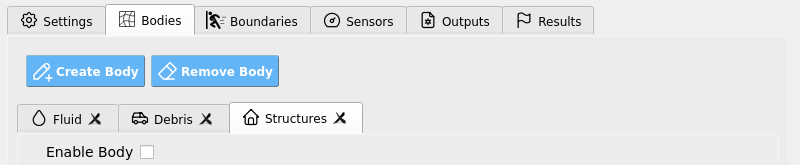
Fig. 4.8.2.4.1 HydroUQ Bodies Structures GUI
Boundaries
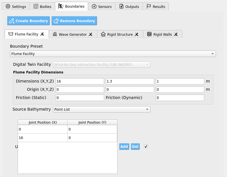
Wave Flume boundary:
Open Boundaries / Flume Facility. We will set the flume boundary to be a rigid body, with a fixed separable velocity condition. Bathymetry joint points should be identical to the ones used in Bodies / Fluid / Geometry.
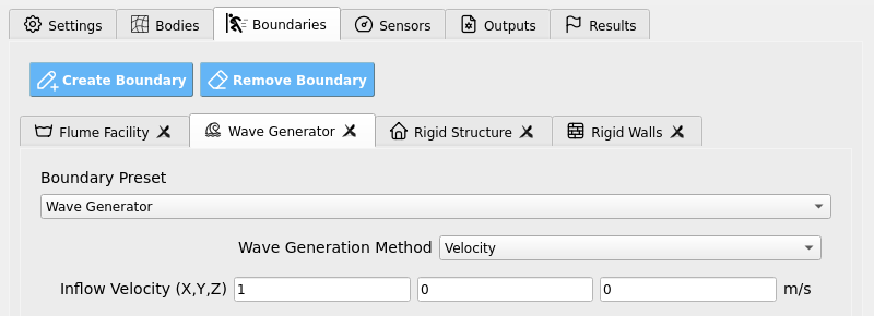
Wave Generator:
Open Boundaries / Wave Generator. Set the method to be “Velocity” as we are replicating the inflow of a pump-driven fluid using a virtually extended flume with a velocity boundary condition.
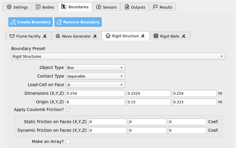
Rigid Structure:
Open Boundaries / Rigid Structure. This is where we will specify the structure as a boundary condition. By doing so, we can determine the exact loads on the rigid boundary grid-nodes, which automatically map to the model defined in the SIM and FEM tab in Steps 3 and 5 for potentially nonlinear UQ structural response analysis.
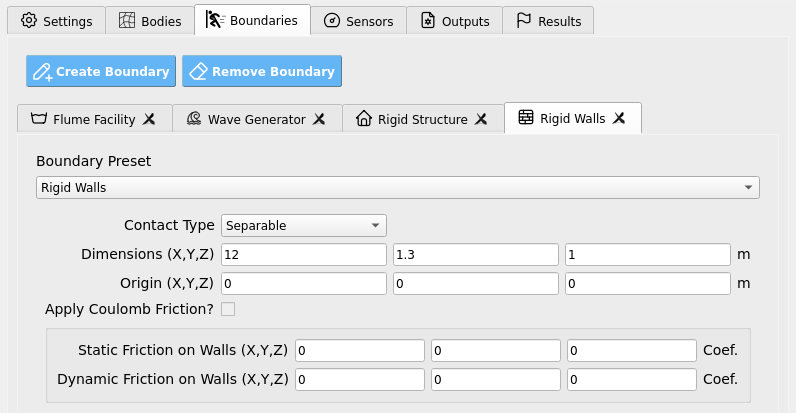
Rigid Walls:
Open Boundaries / Rigid Walls. Set to encompass the flume domain.
Sensors
Wave Gauges:
Open Sensors / Wave Gauges. Set the Use these sensor? box to True so that the simulation will output results for the instruments we set on this page.
Three wave gauges will be defined along the inflow path towards the structural face, where we anticipate a fluid buffer to develop.
Set the origins and dimensions of each wave gauge to encompass at least one grid-cell in each direction as in the table below. To match experimental conditions, we also apply a 30 Hz sampling rate to the wave gauges.
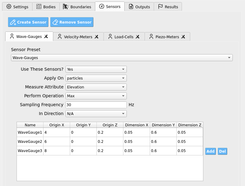
These wave gauges will read all numerical bodies (i.e. particles) within their defined regions at every sampling step and will report the highest elevation value (Position Y) of a contained body as the free-surface elevation at that gauge. The results are written into our sensor results files which we will later analyze.
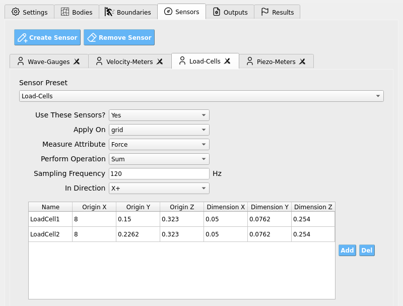
Load Cells:
Open Sensors / Load Cells. Set the Use these sensor? box to True so that the simulation will output results for the instruments we set on this page. Two load cells are defined so that we may map loads onto two nodes of our OpenSees structural model which we defined in Steps 3 and 5. Output frequency is set to 120 Hz to match experiments and capture primary load phenomena.
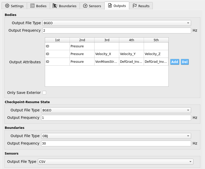
Outputs
Open Outputs. Here we set the non-physical output parameters for the simulation, e.g. attributes to save per frame and file extension types. The particle bodies’ output frequency is set to 2 Hz, meaning the simulation will output results every 0.5 seconds. This is to save disk space and reduce I/O load, but it may be increased if you wish to make animations (e.g., 10 - 30 Hz). Fill the rest of the data in the figure into your GUI to ensure all your outputs match this example. You may alter output attributes if you are an advanced user familiar with ClaymoreUW attributes and wish to perform more advanced analysis.
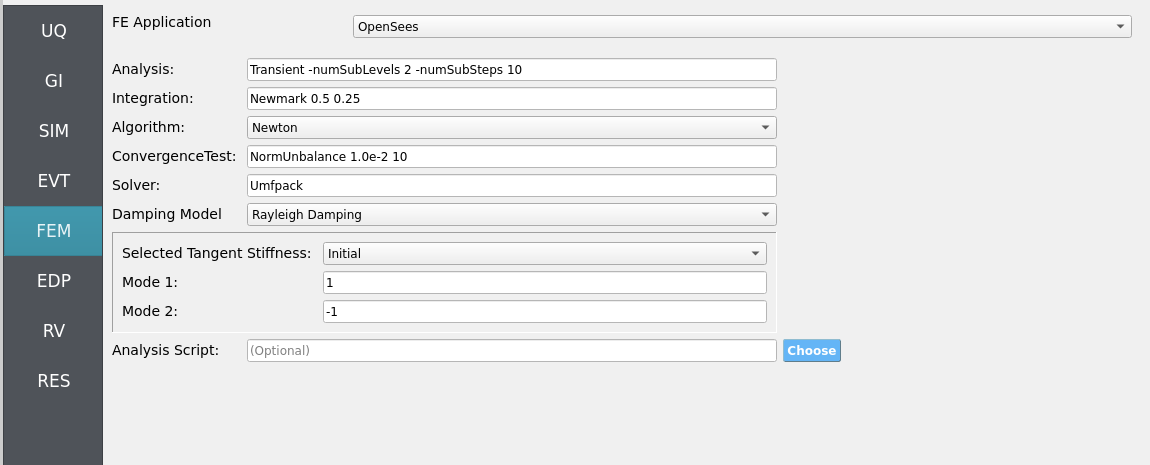
4.8.2.5. Step 5: FEM
This example insofar focused on hydrodynamic forces measured on rigid structures. To perform true structural response analysis, map recovered boundary loads to an OpenSees model in SIM and configure dynamic analysis here as in other HydroUQ tutorials.
Solver: OpenSees dynamic analysis. Check:
Integration step compatible with MPM sensor output interval.
Algorithm/convergence tolerances suitable for expected nonlinearity.
Damping model as needed (e.g., Rayleigh).
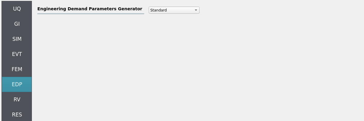
4.8.2.6. Step 6: EDP
Select Engineering Demand Parameters (EDPs) to summarize response:
Peak Floor Acceleration (PFA)
Root Mean Square Acceleration (RMSA)
Peak Floor Displacement (PFD)
Peak Interstory Drift (PID)
Note that other quantities of interest (QoI) are theoretically obtainable from HydroUQ if the custom EDP module is configured by an advanced user. E.g.:
Wave: max free-surface elevation, η, at gauges.
Debris motion: longitudinal displacement (forward/back), lateral spreading angle.
Loads: obstacle force time histories (impact peaks, total impulses).
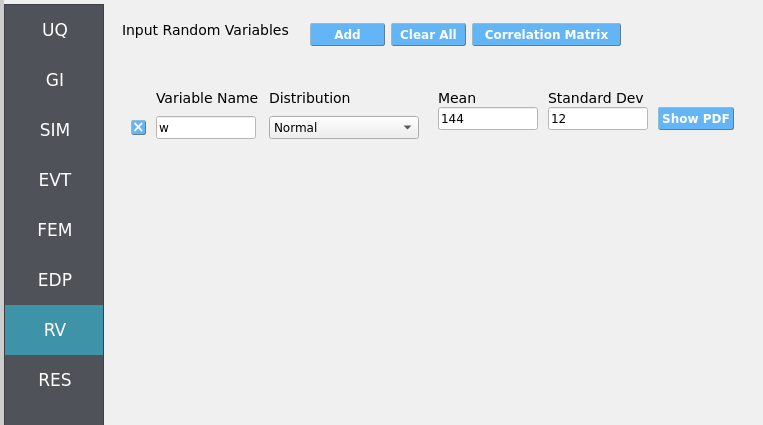
4.8.2.7. Step 7: RV
Define distributions for structural RV:
Structural
w: Normal (mean144, stdev12)
For future UQ, consider:
Debris: mass variance, placement variance.
Wave: steady-state tolerance relative to inflow depth and velocity.
Obstacles: small misalignment/placement tolerance.
4.8.3. Simulation
This case was executed on TACC Stampede3 using 2x NVIDIA H100 GPUs on a single node (queue: h100).
Simulated physical time: 6 seconds. Wall time: 60 minutes (allow ample Max Run Time in job settings).
Important
Provide generous Max Run Time, on the order of 60 to 90 minutes, to complete the run and post-processing before scheduler limits are reached.
Warning
Keep sensor regions, counts, sampling rates, and output frequencies reasonable—excess I/O can dominate runtime.
Outputs
Sensor CSVs (gauges, debris CoM, loads) at your chosen rates.
Particle/field snapshots (e.g., BGEO/VTK) for visualization/diagnostics.
4.8.4. Analysis
Accessing Results and Simulation Files
When the simulation job has been completed, the results and simulation files will be available on the remote system for retrieval or remote post-processing.
Retrieving the results.zip, templatedir.zip, workdir.tar.gz, and MPM folders will allow you to analyze all of the simulation output (e.g., hydrodynamic, structural, uncertainty quantification).
results.zip: Contains primary uncertainty quantification output and MPM sensor files. This will be the primary place for analysis.templatedir.zip: Contains template and workflow files for the job. This is an important resource for debugging your workflows.workdir.tar.gz: Contains the working directories in which each unique simulation was ran. This is where structural response uncertainty is expanded on typically.MPM: Contains all the MPM simulation files. Includes the raw particle output frames which can be used to create animations or to perform more advanced post-processing.
The most straightforward way to retrieve the most important files, results.zip and templatedir.zip, is by clicking the GET From DesignSafe button in HydroUQ.

Fig. 4.8.4.1 HydroUQ GET From DesignSafe button, which opens up a jobs table of all your remote simulations.
Then, right-click on your job (if it is finished) and select Retrieve Data. This will download results.zip and templatedir.zip.
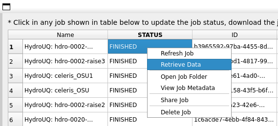
Fig. 4.8.4.2 Locating the Retrieve Data button in the HydroUQ remote jobs table.
HydroUQ will then automatically unzip them into results and templatedir, which will be located in {your_path}/HydroUQ/RemoteWorkDir/tmp.SimCenter. On most systems, this will be ~/Documents/HydroUQ/RemoteWorkDir/tmp.SimCenter, but you can check by clicking on Files / Preferences on the upper-left corner of HydroUQ.
To retrieve workdir.tar.gz and MPM, there are two approaches:
You can right-click on your job within HydroUQ and select
Open Job Folderto be taken directly to the Design Safe web-page displaying all remote files.
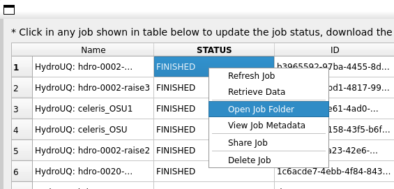
Fig. 4.8.4.3 Locating the Open Job Folder button in the HydroUQ remote jobs table.
You can manually navigate to the designsafe-ci.org website. For the latter, login and go to
Upper-right Drop-down/Job Status.

Fig. 4.8.4.4 Locating the job files on DesignSafe
Check if the job has finished in the central vertical drawer by refreshing the page. If it has, click View Details.
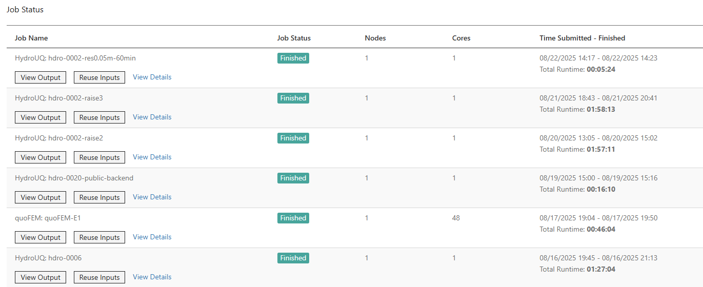
Fig. 4.8.4.5 Job status is finished on DesignSafe
Once the job is finished, the output files should be available in the directory which the analysis results were sent to
Find the files by clicking View Output.
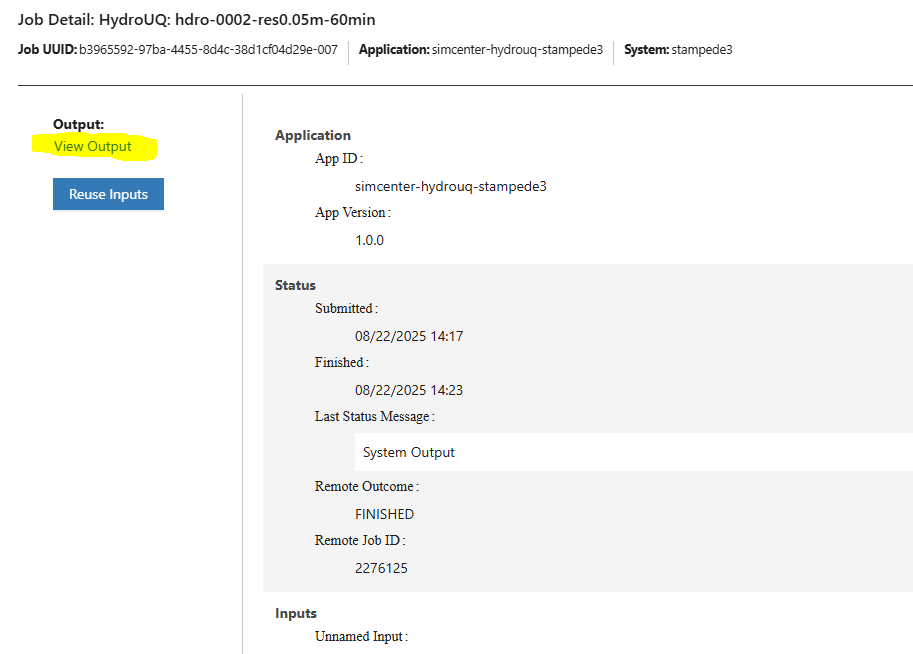
Fig. 4.8.4.6 Viewing the job files on DesignSafe
After navigating to your job folder by one of two ways, it is time to move files for processing. Move important files to somewhere in My Data/ for easier processing. Use the extractor tool available on DesignSafe to unzip the results.zip, workdir.tar.gz, and templatedir.zip folders natively on DesignSafe.
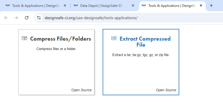
Fig. 4.8.4.7 Extracting the results.zip folder on DesignSafe
Alternatively, you may directly download the zipped folders to your PC, which will require you to use the DesignSafe zip tool on the MPM folder prior.
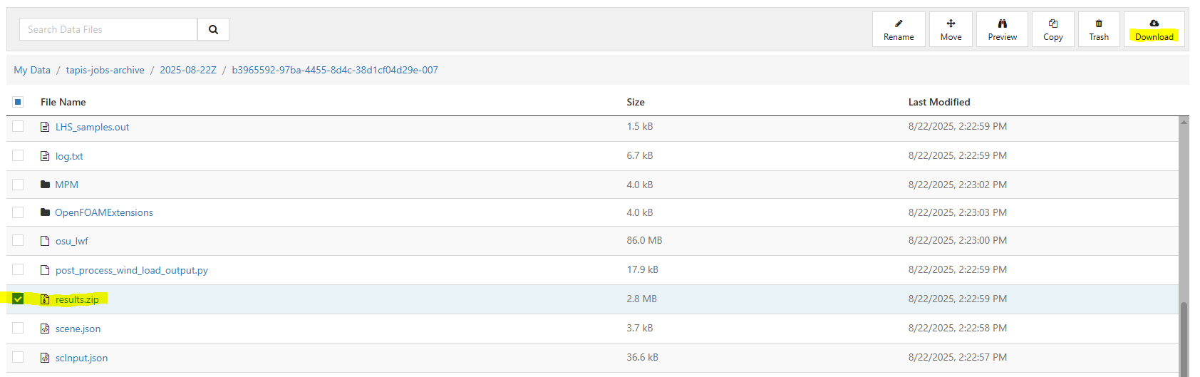
Fig. 4.8.4.8 Download button on DesignSafe shown in red
Locate the downloaded zip folders and extract them somewhere convenient. The HydroUQ local or remote work directory on your computer is a good option.
Warning
Files in the HydroUQ local and remote working directories may be erased if another simulation is set up in HydroUQ, so keep a backup if you wish to maintain the files.
Particle geometry files often have a BGEO extension and are located in the MPM folder. Open with Side FX Houdini Apprentice (free to use) to look at MPM results in high-detail, or use the PartIO library.
HydroUQ’s sensor/probe/instrument output is available in {your_path}/HydroUQ/RemoteWorkDir/tmp.SimCenter/results/ as CSV files. You may process these files as you wish, most opt to use custom Python scripts or Excel due to their simplicity.
Note
For convenience, HydroUQ also includes basic plotting of all sensors files in the EVT / Results tab. Click Post-Process Sensors, configure the drop-down boxes for the sensor you wish to view, and then click Plot.
Plotting the wave gauges shows the development of a tsunami-like wave as it propagates inflow velocity condition over the flat flume bathymetry.
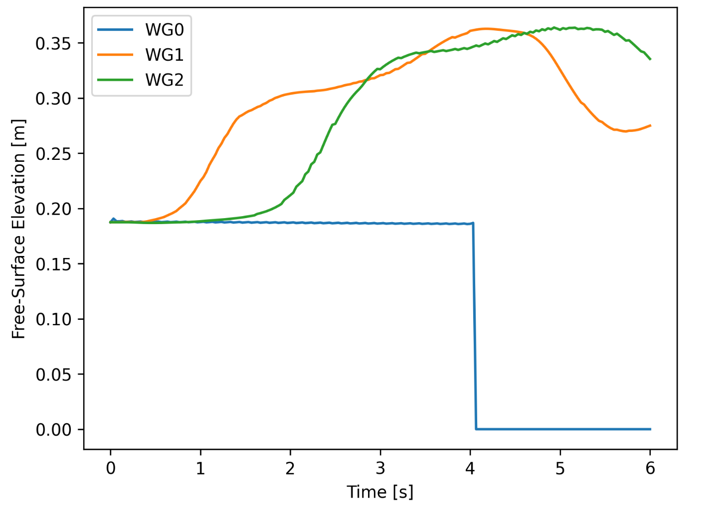
Fig. 4.8.4.9 Simulated free-surface elevations at three wave gauges in MPM.
Load-cell data shows a small initial peak force from debris impact which has been heavily buffered by fluid build-up at the structural face (in-part due to the Froude scale we are operating on relative to debris size), followed by damming forces and eventually a fully developed hydrodynamic drag.
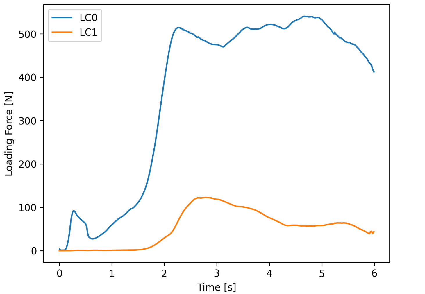
Fig. 4.8.4.10 Simulated load-cell forces in MPM. These are later mapped onto an OpenSees structure for dynamic response analysis.
Structural Analysis
Returning to our primary HydroUQ workflow, which concerns uncertainty in structural response, we may now view the final results in the RES tab. Clicking Summary on the top-bar, a statistical summary of results is shown below:
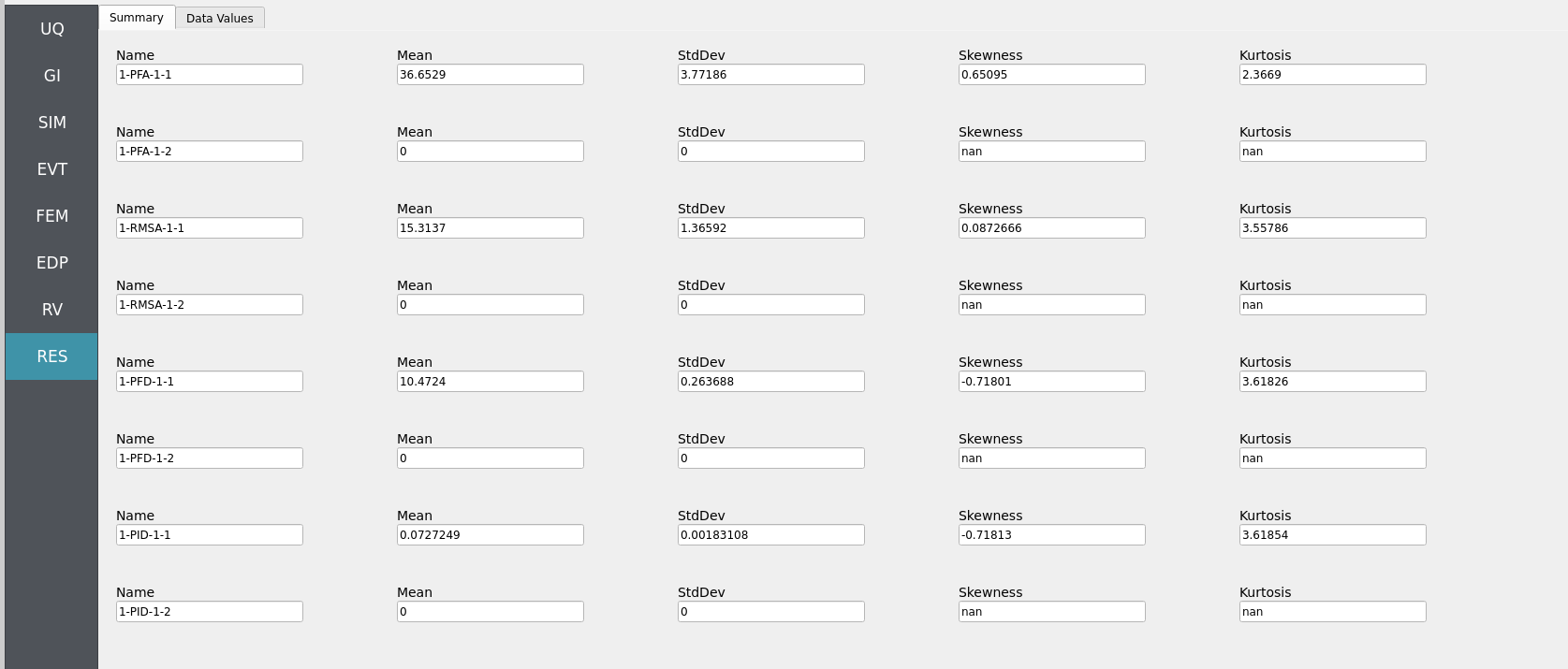
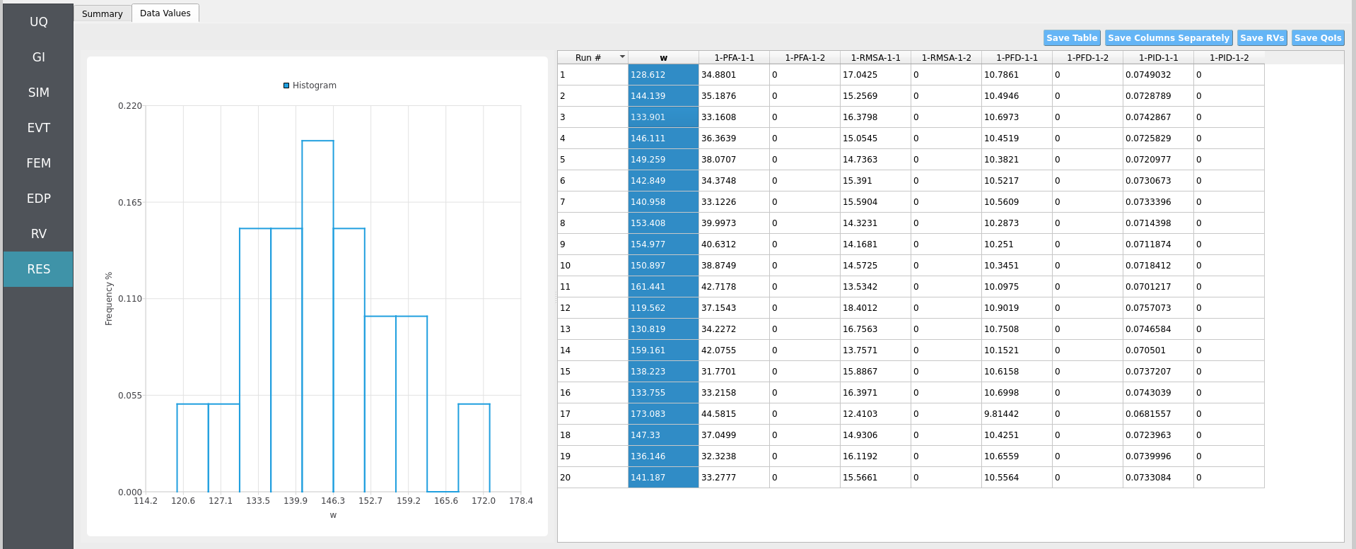
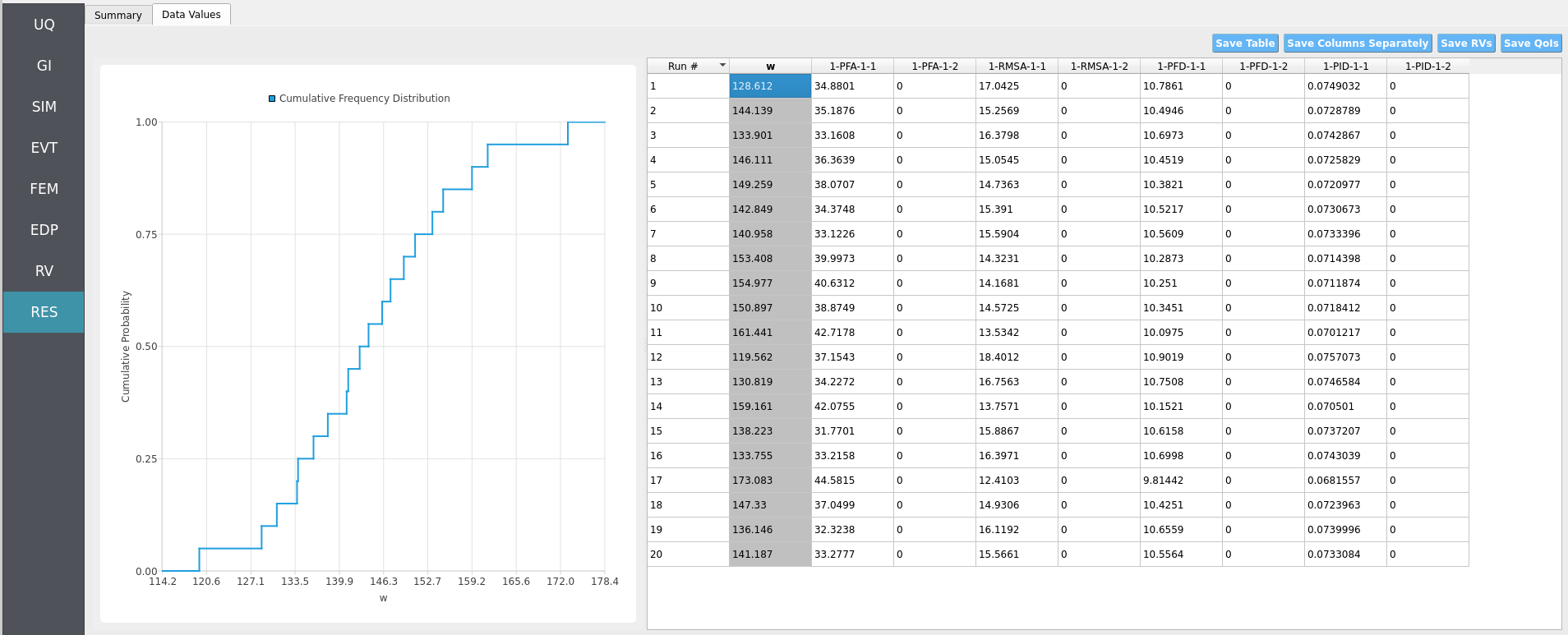
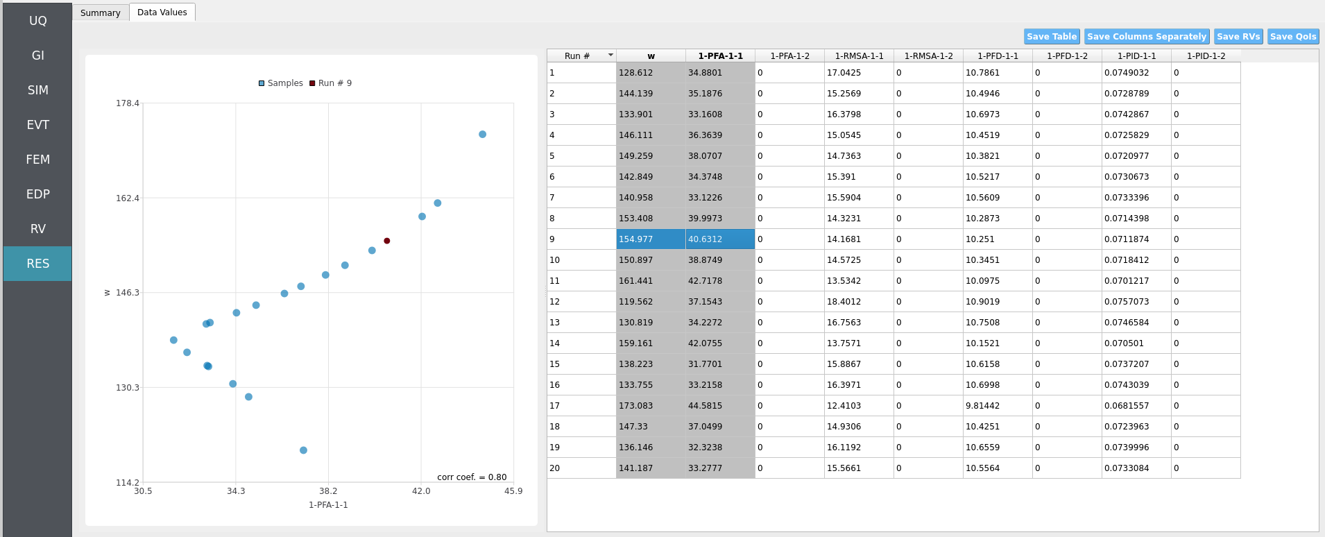
Clicking Data Values on the top-bar shows detailed histograms, cumulative distribution functions, and scatter plots relating the dependent and independent variables:
Note
In the Data Values tab, left- and right-click column headers to change plot axes; selecting a single column with both clicks displays frequency and CDF plots.
Note
Use consistent Froude similitude scaling when comparing numerical simulations, experiments, and full-scale scenarios. For cross-method comparisons, adopt identical debris footprints, friction models, probe placement, and other pertinent parameters to reduce bias.
For more advanced analysis, export results as a CSV file by clicking Save Table on the upper-right of the application window. This will save the independent and dependent variable data. I.e., the Random Variables you defined and the Engineering Demand Parameters determined from the structural response per each simulation.
To save your simulation configuration with results included, click File / Save As and specify a location for the HydroUQ JSON input file to be recorded to. You may then reload the file at a later time by clicking File / Open. You may also send it to others by email or place it in an online repository for research reproducibility. This example’s input file is viewable at Reproducibility.
To directly share your simulation job and results in HydroUQ with other DesignSafe users, click GET from DesignSafe. Then, navigate to the row with your job and right-click it. Select Share Job. You may then enter the DesignSafe username or usernames (comma-separated) to share with.
Important
Sharing a job requires that the job was initially ran with an Archive System ID (listed in the GET from DesignSafe table’s columns) that is not designsafe.storage.default. Any other Archive System ID allows for sharing with DesignSafe members on the associated project. See Jobs for more details.
4.8.5. Conclusions
The HydroUQ MPM digital flume of UW WASIRF reproduces the mechanistic signatures anticipated for steady-flow debris impacts and aligns with the broader tsunami debris literature for the length and time-scale studied.
Motivated readers may wish to extrapolate on this example, attempting to:
Measure \(Fr\) upstream; compute \(C_F\), \(J^*\), and \(R_{PP}\); relate them to \(\Phi\) and \(\beta\).
Build response surfaces \((C_F, J^*) = f(Fr, \Phi, \beta, h_f)\) and propagate Forward UQ over depth–velocity targets and debris arrangement.
Align signal processing with the lab (filter bands, sampling) to separate debris impulses from facility noise.
For design-leaning studies, summarize outcomes as dimensionless fragility envelopes versus \(Fr\) and \(\beta\).
4.8.6. References
Lewis, N. S., Winter, A. O., Bonus, J., Motley, M. R., Eberhard, M. O., Arduino, P., & Lehman, D. E. (2023). Open-source simulation of strongly-coupled fluid-structure interaction between non-conformal interfaces. Frontiers in Built Environment, 9. https://doi.org/10.3389/fbuil.2023.1120518
Lewis, N. (2023). Development of An Open-Source Methodology for Simulation of Civil Engineering Structures Subject to Multi-Hazards. PhD thesis. University of Washington, Seattle.
Bonus, Justin (2023). “Evaluation of Fluid-Driven Debris Impacts in a High-Performance Multi-GPU Material Point Method.” PhD thesis. University of Washington, Seattle.
Bonus, J., & Arduino, P. (2025). ClaymoreUW. Zenodo. https://doi.org/10.5281/zenodo.15128706
4.8.7. Reproducibility
Random seed(s):
1(set in UQ)App version: HydroUQ v4.2.0 (or current)
Solver: MPM (ClaymoreUW, multi-GPU)
Hardware: TACC Lonestar6 or Stampede3, 3x A100 or 4x H100 (single node,
gpu-a100orh100queue)Simulated time: 6 seconds; Wall time: 1 hour
Sensor sampling: wave-gauges 120 Hz; particle output 2-10 Hz
Input: The HydroUQ input file is as follows: input.json , is used:
Click to expand the HydroUQ input file used for this example
1{
2 "Applications": {
3 "EDP": {
4 "Application": "StandardEDP",
5 "ApplicationData": {
6 }
7 },
8 "Events": [
9 {
10 "Application": "MPM",
11 "ApplicationData": {
12 },
13 "EventClassification": "Hydro",
14 "defaultMaxRunTime": "1440",
15 "driverFile": "sc_driver",
16 "inputFile": "scInput.json",
17 "maxRunTime": "120",
18 "programFile": "osu_lwf",
19 "publicDirectory": "./"
20 }
21 ],
22 "Modeling": {
23 "Application": "MDOF_BuildingModel",
24 "ApplicationData": {
25 }
26 },
27 "Simulation": {
28 "Application": "OpenSees-Simulation",
29 "ApplicationData": {
30 }
31 },
32 "UQ": {
33 "Application": "Dakota-UQ",
34 "ApplicationData": {
35 }
36 }
37 },
38 "DefaultValues": {
39 "driverFile": "driver",
40 "edpFiles": [
41 "EDP.json"
42 ],
43 "filenameAIM": "AIM.json",
44 "filenameDL": "BIM.json",
45 "filenameEDP": "EDP.json",
46 "filenameEVENT": "EVENT.json",
47 "filenameSAM": "SAM.json",
48 "filenameSIM": "SIM.json",
49 "rvFiles": [
50 "AIM.json",
51 "SAM.json",
52 "EVENT.json",
53 "SIM.json"
54 ],
55 "workflowInput": "scInput.json",
56 "workflowOutput": "EDP.json"
57 },
58 "EDP": {
59 "type": "StandardEDP"
60 },
61 "Events": [
62 {
63 "Application": "MPM",
64 "EventClassification": "Hydro",
65 "example": "UW WASIRF",
66 "bodies": [
67 {
68 "algorithm": {
69 "ASFLIP_alpha": 0,
70 "ASFLIP_beta_max": 0,
71 "ASFLIP_beta_min": 0,
72 "FBAR_fused_kernel": true,
73 "FBAR_psi": 0.9,
74 "ppc": 8,
75 "type": "particles",
76 "use_ASFLIP": false,
77 "use_FBAR": true
78 },
79 "geometry": [
80 {
81 "apply_array": false,
82 "apply_rotation": false,
83 "body_preset": "Fluid",
84 "facility": "Wind-Air-Sea Interaction Facility (UW WASIRF)",
85 "facility_dimensions": [
86 12.2,
87 1.3,
88 1.0
89 ],
90 "fill_flume_upto_SWL": true,
91 "object": "Box",
92 "offset": [
93 0,
94 0,
95 0
96 ],
97 "operation": "add",
98 "span": [
99 12.2,
100 0.2,
101 1.0
102 ],
103 "standing_water_level": 0.2,
104 "track_particle_id": [
105 "0"
106 ],
107 "use_custom_bathymetry": false
108 }
109 ],
110 "gpu": 0,
111 "material": {
112 "CFL": 0.5,
113 "bulk_modulus": 210000000,
114 "constitutive": "JFluid",
115 "gamma": 7.15,
116 "material_preset": "Water (Fresh)",
117 "rho": 1000,
118 "viscosity": 0.001
119 },
120 "model": 0,
121 "name": "fluid",
122 "output_attribs": [
123 "ID",
124 "Pressure"
125 ],
126 "partition": [
127 {
128 "gpu": 0,
129 "model": 0,
130 "partition_end": [
131 6.1,
132 1.3,
133 1.0
134 ],
135 "partition_start": [
136 0,
137 0,
138 0
139 ]
140 },
141 {
142 "gpu": 1,
143 "model": 0,
144 "partition_end": [
145 12.2,
146 1.3,
147 1.0
148 ],
149 "partition_start": [
150 6.1,
151 0,
152 0
153 ]
154 },
155 {
156 "gpu": 2,
157 "model": 0,
158 "partition_end": [
159 18.3,
160 1.3,
161 1.0
162 ],
163 "partition_start": [
164 12.2,
165 0,
166 0
167 ]
168 }
169 ],
170 "partition_end": [
171 6.1,
172 1.3,
173 1.0
174 ],
175 "partition_start": [
176 0,
177 0,
178 0
179 ],
180 "target_attribs": [
181 "Position_Y"
182 ],
183 "track_attribs": [
184 "Position_X",
185 "Position_Z",
186 "Pressure"
187 ],
188 "track_particle_id": [
189 0
190 ],
191 "type": "particles",
192 "velocity": [
193 1,
194 0,
195 0
196 ]
197 },
198 {
199 "algorithm": {
200 "ASFLIP_alpha": 0,
201 "ASFLIP_beta_max": 0,
202 "ASFLIP_beta_min": 0,
203 "FBAR_fused_kernel": true,
204 "FBAR_psi": 0,
205 "ppc": 8,
206 "type": "particles",
207 "use_ASFLIP": true,
208 "use_FBAR": false
209 },
210 "geometry": [
211 {
212 "apply_array": true,
213 "apply_rotation": true,
214 "array": [
215 3,
216 1,
217 1
218 ],
219 "body_preset": "Debris",
220 "facility": "Wind-Air-Sea Interaction Facility (UW WASIRF)",
221 "facility_dimensions": [
222 12.2,
223 1.3,
224 1.0
225 ],
226 "fulcrum": [
227 0,
228 0,
229 0
230 ],
231 "object": "Box",
232 "offset": [
233 5.0,
234 0.2,
235 0.5
236 ],
237 "operation": "add",
238 "rotate": [
239 0,
240 0,
241 0
242 ],
243 "spacing": [
244 0.5,
245 0.01,
246 0.01
247 ],
248 "span": [
249 0.2,
250 0.05,
251 0.05
252 ],
253 "track_particle_id": [
254 "0"
255 ]
256 }
257 ],
258 "gpu": 0,
259 "material": {
260 "CFL": 0.5,
261 "constitutive": "FixedCorotated",
262 "material_preset": "Plastic",
263 "poisson_ratio": 0.3,
264 "rho": 981,
265 "youngs_modulus": 100000000
266 },
267 "model": 1,
268 "name": "debris",
269 "output_attribs": [
270 "ID",
271 "Pressure",
272 "Velocity_X",
273 "Velocity_Y",
274 "Velocity_Z"
275 ],
276 "partition": [
277 {
278 "gpu": 0,
279 "model": 1,
280 "partition_end": [
281 12.2,
282 1.3,
283 1.0
284 ],
285 "partition_start": [
286 0,
287 0,
288 0
289 ]
290 }
291 ],
292 "partition_end": [
293 12.2,
294 1.3,
295 1.0
296 ],
297 "partition_start": [
298 0,
299 0,
300 0
301 ],
302 "target_attribs": [
303 "Position_Y"
304 ],
305 "track_attribs": [
306 "Position_X",
307 "Position_Z",
308 "Pressure"
309 ],
310 "track_particle_id": [
311 0
312 ],
313 "type": "particles",
314 "velocity": [
315 1.0,
316 0,
317 0
318 ]
319 },
320 {
321 "algorithm": {
322 "ASFLIP_alpha": 0,
323 "ASFLIP_beta_max": 0,
324 "ASFLIP_beta_min": 0,
325 "FBAR_fused_kernel": true,
326 "FBAR_psi": 0.9,
327 "ppc": 8,
328 "type": "particles",
329 "use_ASFLIP": false,
330 "use_FBAR": true
331 },
332 "geometry": [
333 {
334 "apply_array": false,
335 "apply_rotation": false,
336 "body_preset": "Fluid",
337 "facility": "Wind-Air-Sea Interaction Facility (UW WASIRF)",
338 "facility_dimensions": [
339 12.2,
340 1.3,
341 1.0
342 ],
343 "fill_flume_upto_SWL": true,
344 "object": "Box",
345 "offset": [
346 0,
347 0,
348 0
349 ],
350 "operation": "add",
351 "span": [
352 12.2,
353 0.2,
354 1.0
355 ],
356 "standing_water_level": 0.2,
357 "track_particle_id": [
358 "0"
359 ],
360 "use_custom_bathymetry": false
361 }
362 ],
363 "gpu": 1,
364 "material": {
365 "CFL": 0.5,
366 "bulk_modulus": 210000000,
367 "constitutive": "JFluid",
368 "gamma": 7.15,
369 "material_preset": "Water (Fresh)",
370 "rho": 1000,
371 "viscosity": 0.001
372 },
373 "model": 0,
374 "name": "fluid",
375 "output_attribs": [
376 "ID",
377 "Pressure"
378 ],
379 "partition": [
380 {
381 "gpu": 0,
382 "model": 0,
383 "partition_end": [
384 6.1,
385 1.3,
386 1.0
387 ],
388 "partition_start": [
389 0,
390 0,
391 0
392 ]
393 },
394 {
395 "gpu": 1,
396 "model": 0,
397 "partition_end": [
398 12.2,
399 1.3,
400 1.0
401 ],
402 "partition_start": [
403 6.1,
404 0,
405 0
406 ]
407 },
408 {
409 "gpu": 2,
410 "model": 0,
411 "partition_end": [
412 18.3,
413 1.3,
414 1.0
415 ],
416 "partition_start": [
417 12.2,
418 0,
419 0
420 ]
421 }
422 ],
423 "partition_end": [
424 12.2,
425 1.3,
426 1.0
427 ],
428 "partition_start": [
429 6.1,
430 0,
431 0
432 ],
433 "target_attribs": [
434 "Position_Y"
435 ],
436 "track_attribs": [
437 "Position_X",
438 "Position_Z",
439 "Pressure"
440 ],
441 "track_particle_id": [
442 0
443 ],
444 "type": "particles",
445 "velocity": [
446 1,
447 0,
448 0
449 ]
450 },
451 {
452 "algorithm": {
453 "ASFLIP_alpha": 0,
454 "ASFLIP_beta_max": 0,
455 "ASFLIP_beta_min": 0,
456 "FBAR_fused_kernel": true,
457 "FBAR_psi": 0.9,
458 "ppc": 8,
459 "type": "particles",
460 "use_ASFLIP": false,
461 "use_FBAR": true
462 },
463 "geometry": [
464 {
465 "apply_array": false,
466 "apply_rotation": false,
467 "body_preset": "Fluid",
468 "facility": "Wind-Air-Sea Interaction Facility (UW WASIRF)",
469 "facility_dimensions": [
470 12.2,
471 1.3,
472 1.0
473 ],
474 "fill_flume_upto_SWL": true,
475 "object": "Box",
476 "offset": [
477 0,
478 0,
479 0
480 ],
481 "operation": "add",
482 "span": [
483 12.2,
484 0.2,
485 1.0
486 ],
487 "standing_water_level": 0.2,
488 "track_particle_id": [
489 "0"
490 ],
491 "use_custom_bathymetry": false
492 }
493 ],
494 "gpu": 2,
495 "material": {
496 "CFL": 0.5,
497 "bulk_modulus": 210000000,
498 "constitutive": "JFluid",
499 "gamma": 7.15,
500 "material_preset": "Water (Fresh)",
501 "rho": 1000,
502 "viscosity": 0.001
503 },
504 "model": 0,
505 "name": "fluid",
506 "output_attribs": [
507 "ID",
508 "Pressure"
509 ],
510 "partition": [
511 {
512 "gpu": 0,
513 "model": 0,
514 "partition_end": [
515 6.1,
516 1.3,
517 1.0
518 ],
519 "partition_start": [
520 0,
521 0,
522 0
523 ]
524 },
525 {
526 "gpu": 1,
527 "model": 0,
528 "partition_end": [
529 12.2,
530 1.3,
531 1.0
532 ],
533 "partition_start": [
534 6.1,
535 0,
536 0
537 ]
538 },
539 {
540 "gpu": 2,
541 "model": 0,
542 "partition_end": [
543 18.3,
544 1.3,
545 1.0
546 ],
547 "partition_start": [
548 12.2,
549 0,
550 0
551 ]
552 }
553 ],
554 "partition_end": [
555 18.3,
556 1.3,
557 1.0
558 ],
559 "partition_start": [
560 12.2,
561 0,
562 0
563 ],
564 "target_attribs": [
565 "Position_Y"
566 ],
567 "track_attribs": [
568 "Position_X",
569 "Position_Z",
570 "Pressure"
571 ],
572 "track_particle_id": [
573 0
574 ],
575 "type": "particles",
576 "velocity": [
577 1,
578 0,
579 0
580 ]
581 }
582 ],
583 "boundaries": [
584 {
585 "contact": "Separable",
586 "domain_end": [
587 16.0,
588 1.3,
589 1.0
590 ],
591 "domain_start": [
592 0,
593 0,
594 0
595 ],
596 "friction_dynamic": 0,
597 "friction_static": 0,
598 "object": "Bathymetry",
599 "use_custom_bathymetry": true,
600 "bathymetry": [[0,0], [16.0,0]]
601 },
602 {
603 "contact": "Separable",
604 "domain_end": [
605 4.0,
606 1.3,
607 1.0
608 ],
609 "domain_start": [
610 0,
611 0,
612 0
613 ],
614 "velocity": [
615 1,
616 0,
617 0
618 ],
619 "friction_dynamic": 0,
620 "friction_static": 0,
621 "object": "Velocity"
622 },
623 {
624 "contact": "Separable",
625 "domain_end": [
626 8.254,
627 0.3024,
628 0.577
629 ],
630 "domain_start": [
631 8,
632 0.15,
633 0.323
634 ],
635 "friction_dynamic": 0,
636 "friction_static": 0,
637 "object": "Box"
638 },
639 {
640 "contact": "Separable",
641 "domain_end": [
642 12,
643 1.3,
644 1.0
645 ],
646 "domain_start": [
647 0,
648 0,
649 0
650 ],
651 "friction_dynamic": 0,
652 "friction_static": 0,
653 "object": "Walls"
654 }
655 ],
656 "computer": {
657 "hpc": "TACC - UT Austin - Lonestar6",
658 "hpc_card_architecture": "Ampere",
659 "hpc_card_brand": "NVIDIA",
660 "hpc_card_compute_capability": 80,
661 "hpc_card_global_memory": 40,
662 "hpc_card_name": "A100",
663 "hpc_queue": "gpu-a100",
664 "models_per_gpu": 3,
665 "num_gpus": 3
666 },
667 "grid-sensors": [
668 {
669 "attribute": "Force",
670 "direction": "X+",
671 "domain_end": [
672 8.05,
673 0.2262,
674 0.577
675 ],
676 "domain_start": [
677 8,
678 0.15,
679 0.323
680 ],
681 "name": "LoadCell1",
682 "operation": "Sum",
683 "output_frequency": 120,
684 "preset": "Load-Cells",
685 "summary": [
686 [
687 "LoadCell1",
688 8,
689 0.15,
690 0.323,
691 0.05,
692 0.0762,
693 0.254
694 ],
695 [
696 "LoadCell2",
697 8,
698 0.2262,
699 0.323,
700 0.05,
701 0.0762,
702 0.254
703 ]
704 ],
705 "toggle": true,
706 "type": "grid"
707 },
708 {
709 "attribute": "Force",
710 "direction": "X+",
711 "domain_end": [
712 8.05,
713 0.3024,
714 0.577
715 ],
716 "domain_start": [
717 8,
718 0.2262,
719 0.323
720 ],
721 "name": "LoadCell2",
722 "operation": "Sum",
723 "output_frequency": 120,
724 "preset": "Load-Cells",
725 "summary": [
726 [
727 "LoadCell1",
728 8,
729 0.15,
730 0.323,
731 0.05,
732 0.0762,
733 0.254
734 ],
735 [
736 "LoadCell2",
737 8,
738 0.2262,
739 0.323,
740 0.05,
741 0.0762,
742 0.254
743 ]
744 ],
745 "toggle": true,
746 "type": "grid"
747 }
748 ],
749 "outputs": {
750 "bodies_output_freq": 2,
751 "bodies_save_suffix": "BGEO",
752 "boundaries_output_freq": 30,
753 "boundaries_save_suffix": "OBJ",
754 "checkpoints_output_freq": 1,
755 "checkpoints_save_suffix": "BGEO",
756 "energies_output_freq": 30,
757 "energies_save_suffix": "CSV",
758 "output_attribs": [
759 [
760 "ID",
761 "Pressure"
762 ],
763 [
764 "ID",
765 "Pressure",
766 "Velocity_X",
767 "Velocity_Y",
768 "Velocity_Z"
769 ],
770 [
771 "ID",
772 "Pressure",
773 "VonMisesStress",
774 "DefGrad_Invariant2",
775 "DefGrad_Invariant3"
776 ]
777 ],
778 "particles_output_exterior_only": false,
779 "sensors_save_suffix": "CSV",
780 "useKineticEnergy": false,
781 "usePotentialEnergy": false,
782 "useStrainEnergy": false
783 },
784 "particle-sensors": [
785 {
786 "attribute": "Elevation",
787 "direction": "N/A",
788 "domain_end": [
789 4.05,
790 0.6,
791 0.25
792 ],
793 "domain_start": [
794 4,
795 0,
796 0.2
797 ],
798 "name": "WaveGauge1",
799 "operation": "Max",
800 "output_frequency": 30,
801 "preset": "Wave-Gauges",
802 "summary": [
803 [
804 "WaveGauge1",
805 4,
806 0,
807 0.2,
808 0.05,
809 0.6,
810 0.05
811 ],
812 [
813 "WaveGauge2",
814 6,
815 0,
816 0.2,
817 0.05,
818 0.6,
819 0.05
820 ],
821 [
822 "WaveGauge3",
823 8,
824 0,
825 0.2,
826 0.05,
827 0.6,
828 0.05
829 ]
830 ],
831 "toggle": true,
832 "type": "particles"
833 },
834 {
835 "attribute": "Elevation",
836 "direction": "N/A",
837 "domain_end": [
838 6.05,
839 0.6,
840 0.25
841 ],
842 "domain_start": [
843 6,
844 0,
845 0.2
846 ],
847 "name": "WaveGauge2",
848 "operation": "Max",
849 "output_frequency": 30,
850 "preset": "Wave-Gauges",
851 "summary": [
852 [
853 "WaveGauge1",
854 4,
855 0,
856 0.2,
857 0.05,
858 0.6,
859 0.05
860 ],
861 [
862 "WaveGauge2",
863 6,
864 0,
865 0.2,
866 0.05,
867 0.6,
868 0.02
869 ],
870 [
871 "WaveGauge3",
872 8,
873 0,
874 0.2,
875 0.05,
876 0.6,
877 0.05
878 ]
879 ],
880 "toggle": true,
881 "type": "particles"
882 },
883 {
884 "attribute": "Elevation",
885 "direction": "N/A",
886 "domain_end": [
887 8.05,
888 0.6,
889 0.25
890 ],
891 "domain_start": [
892 8,
893 0,
894 0.2
895 ],
896 "name": "WaveGauge3",
897 "operation": "Max",
898 "output_frequency": 30,
899 "preset": "Wave-Gauges",
900 "summary": [
901 [
902 "WaveGauge1",
903 4,
904 0,
905 0.2,
906 0.05,
907 0.6,
908 0.05
909 ],
910 [
911 "WaveGauge2",
912 6,
913 0,
914 0.2,
915 0.05,
916 0.6,
917 0.05
918 ],
919 [
920 "WaveGauge3",
921 8,
922 0,
923 0.2,
924 0.05,
925 0.6,
926 0.05
927 ]
928 ],
929 "toggle": true,
930 "type": "particles"
931 }
932 ],
933 "scaling": {
934 "cauchy_bulk_ratio": 1,
935 "froude_length_ratio": 1,
936 "froude_time_ratio": 1,
937 "use_cauchy_scaling": false,
938 "use_froude_scaling": false
939 },
940 "simulation": {
941 "cauchy_bulk_ratio": 1,
942 "cfl": 0.5,
943 "default_dt": 0.001,
944 "default_dx": 0.05,
945 "domain": [
946 16.0,
947 1.3,
948 1.0
949 ],
950 "duration": 6.0,
951 "fps": 2,
952 "frames": 2,
953 "froude_scaling": 1,
954 "froude_time_ratio": 1,
955 "gravity": [
956 0,
957 -9.80665,
958 0
959 ],
960 "initial_time": 0,
961 "mirror_domain": [
962 false,
963 false,
964 false
965 ],
966 "particles_output_exterior_only": false,
967 "save_suffix": ".bgeo",
968 "time": 0,
969 "time_integration": "Explicit",
970 "use_cauchy_scaling": false,
971 "use_froude_scaling": false
972 },
973 "subtype": "MPM",
974 "type": "MPM"
975 }
976 ],
977 "GeneralInformation": {
978 "NumberOfStories": 1,
979 "PlanArea": 0.064516,
980 "StructureType": "S2",
981 "YearBuilt": 2021,
982 "depth": 0.254,
983 "height": 0.254,
984 "location": {
985 "latitude": 47.6567,
986 "longitude": -122.3066
987 },
988 "name": "Aluminum Box @ UW WASIRF",
989 "planArea": 0.064516,
990 "stories": 1,
991 "units": {
992 "force": "N",
993 "length": "m",
994 "temperature": "C",
995 "time": "sec"
996 },
997 "width": 0.254
998 },
999 "Modeling": {
1000 "Bx": 0.1,
1001 "By": 0.1,
1002 "Fyx": 1000000,
1003 "Fyy": 1000000,
1004 "Krz": 10000000000,
1005 "Kx": 100,
1006 "Ky": 100,
1007 "ModelData": [
1008 {
1009 "Fyx": 1000000,
1010 "Fyy": 1000000,
1011 "Ktheta": 10000000000,
1012 "bx": 0.1,
1013 "by": 0.1,
1014 "height": 144,
1015 "kx": 100,
1016 "ky": 100,
1017 "weight": "RV.w"
1018 }
1019 ],
1020 "dampingRatio": 0.02,
1021 "height": 0.615,
1022 "massX": 0,
1023 "massY": 0,
1024 "numStories": 1,
1025 "randomVar": [
1026 ],
1027 "responseX": 0,
1028 "responseY": 0,
1029 "type": "MDOF_BuildingModel",
1030 "weight": "RV.w"
1031 },
1032 "Simulation": {
1033 "Application": "OpenSees-Simulation",
1034 "algorithm": "Newton",
1035 "analysis": "Transient -numSubLevels 2 -numSubSteps 10",
1036 "convergenceTest": "NormUnbalance 1.0e-2 10",
1037 "dampingModel": "Rayleigh Damping",
1038 "firstMode": 1,
1039 "integration": "Newmark 0.5 0.25",
1040 "modalRayleighTangentRatio": 0,
1041 "numModesModal": -1,
1042 "rayleighTangent": "Initial",
1043 "secondMode": -1,
1044 "solver": "Umfpack"
1045 },
1046 "UQ": {
1047 "parallelExecution": true,
1048 "samplingMethodData": {
1049 "method": "LHS",
1050 "samples": 20,
1051 "seed": 1
1052 },
1053 "saveWorkDir": true,
1054 "uqType": "Forward Propagation"
1055 },
1056 "correlationMatrix": [
1057 1
1058 ],
1059 "localAppDir": "/home/justinbonus/SimCenter/HydroUQ/build",
1060 "randomVariables": [
1061 {
1062 "distribution": "Normal",
1063 "inputType": "Parameters",
1064 "mean": 144,
1065 "name": "w",
1066 "refCount": 1,
1067 "stdDev": 12,
1068 "value": "RV.w",
1069 "variableClass": "Uncertain"
1070 }
1071 ],
1072 "remoteAppDir": "/home/justinbonus/SimCenter/HydroUQ/build",
1073 "resultType": "SimCenterUQResultsSampling",
1074 "runType": "runningLocal",
1075 "summary": [
1076 ],
1077 "workingDir": "/home/justinbonus/Documents/HydroUQ/LocalWorkDir"
1078}