2.7. ANA: Asset Analysis

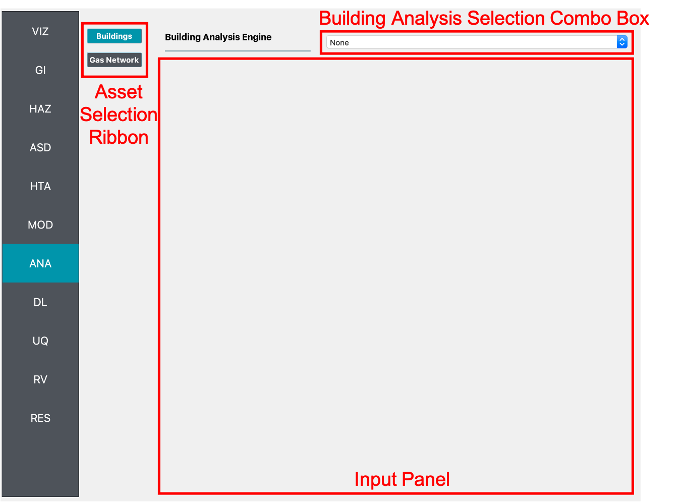
In this panel, users can select specific applications for analyzing different asset classes. To choose an asset type, such as Buildings or Transportation Network, users interact with the Asset Selection Ribbon on the left side of the interface as depicted in Fig. 2.7.1. This ribbon is initially hidden and becomes visible when multiple asset types are selected in the GI: General Information panel. Only assets marked in the GI panel will be listed in the Asset Selection Ribbon. Switching between assets updates the Input Panel to display the relevant analysis applications for the selected asset type.

Fig. 2.7.1 Buildings analysis input panel.

2.7.1. Buildings

For building analysis, the following applications are supported:

• OpenSees

• OpenSeesPy

• IMasEDP

• Capacity Spectrum Method

• PreTrained Surrogate Models

• CustomPy-Simulation

• None

2.7.1.1. OpenSees Analysis Model

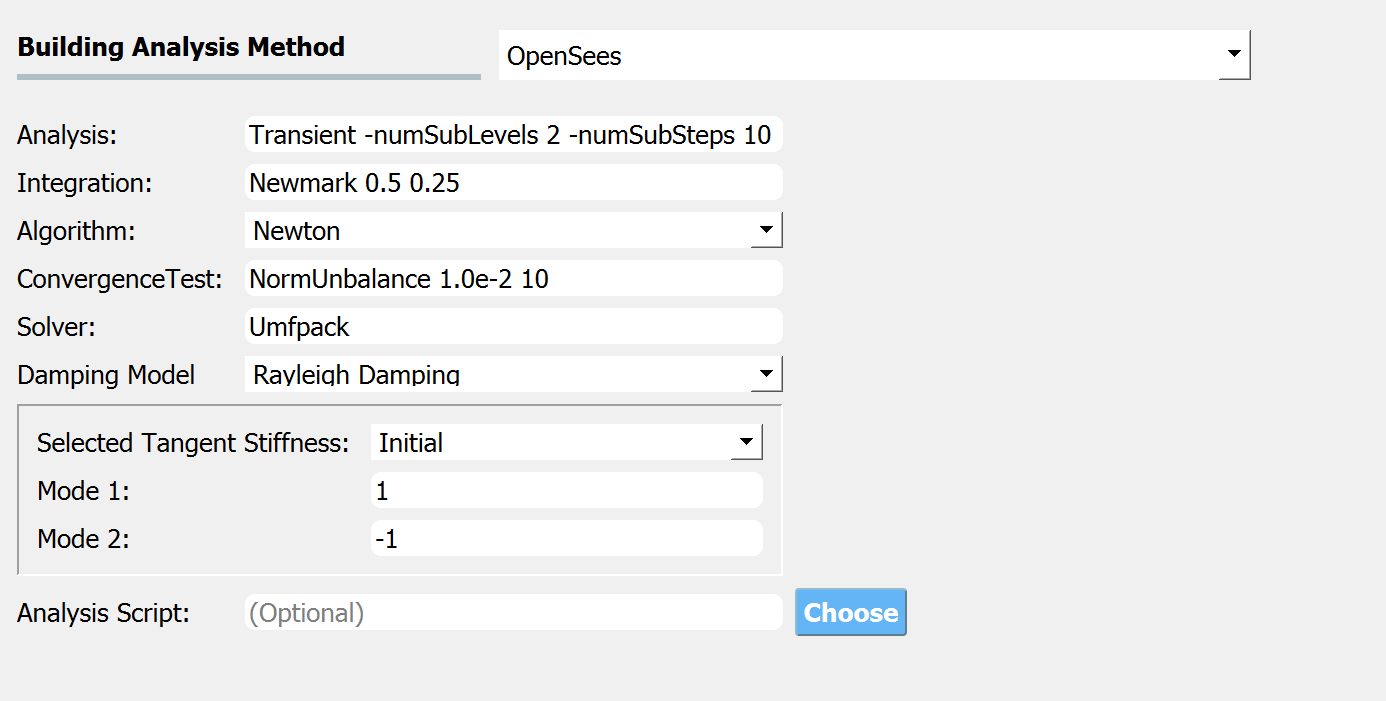
The OpenSees option performs structural analysis using OpenSees. If an “Analysis Script” argument is provided, the quantities defined with the graphical user interface will be ignored.

Fig. 2.7.1.1.1 OpenSees analysis option

Following is an example of user-provided analysis script (.tcl) that additionally sets the “-fullGenLapack 1” flag on top of the selections shown in the above image.

# Perform the analysis
numberer RCM
constraints Transformation
system Umfpack
integrator Newmark 0.5 0.25
test NormUnbalance 1.0e-2 10 
algorithm Newton
analysis Transient -numSubLevels 2 -numSubSteps 10
#set lambdaN [eigen 1];
set lambdaN [eigen -fullGenLapack 1]
set lambda1 [lindex $lambdaN 0]

set T1 [expr 2*3.14159/$lambda1]
set dTana [expr $T1/20.]
if {$dt < $dTana} {set dTana $dt}
analyze [expr int($numStep*$dt/$dTana)] $dTana 
remove recorders 

2.7.1.2. OpenSeesPy Analysis Model

The OpenSeesPy application utilizes OpenSeesPy for structural analysis.

2.7.1.3. IMasEDP Analysis Model

The IMasEDP application directly uses the hazard intensity measure (IM) as the engineering demand parameter (EDP), bypassing structural analysis.

2.7.1.4. Capacity Spectrum Method

The Capacity Spectrum Method is a simplified method for estimating the seismic performance of structures. The method uses the capacity curve of the structure and the response spectrum of the ground motion to estimate the maximum response of the structure. The method is based on the assumption that the maximum response of the structure is the intersection of the capacity curve and the response spectrum. The method requires three inputs: the demand spectrum, the capacity curve, and the damping model.

Demand Spectrum Model:

The demand spectrum model is the response spectrum of the ground motion assuming a 5% damping ratio. The demand spectrum model defined in HAZUS [HAZUS2022] is implemented in R2D now. This model uses pesudo-spectrum acceleration at 0.3 seconds and 1.0 seonds as the anchor points and completes the spectrum using the method described in section 4.1.3.2 of [HAZUS2022], considering the earthquake magnitude.

To use the HAZUS demand spectrum model, “SA_0.3” and “SA_1.0” should exist in the columns of the ground motion intensity measures defined in the ASD tab. Other demand spectrum model can be implemented by editing SimCenterBackendApplication Python script here or contacting the developers.

HAZUS2022(1,2,3,4,5,6,7,8,9)

Federal Emergency Management Agency (FEMA) (2022) Hazus Multi-Hazard Loss Estimation Methodology: Earthquake Model (Hazus®-MH . Technical Manual 5.1). Washington, DC: Mitigation Division, Department of Homeland Security, Federal Emergency Management Agency.

Capacity Curve Model:

The capacity curve model proposed by Cao and Peterson [cao2006] is implemented in R2D. The model is an extension of the [HAZUS2022] capacity curve model. The model uses the capacity curve parameters (e.g. yield strength, yield displacement, ultimate strength, ultimate displacement etc.) to anchor the capacity curve of the structure. Further, an ecliptic passing the yield and ultimate points in [HAZUS2022] is used to complete the capacity curve. To use this model, all building information needed to classfify the building into a class defined in [HAZUS2022] should be provided in the ASD tab. R2D Example 1 provides an example of how to define the building inventory for the capacity curve model.

The model is implemented in the SimCenterBackendApplication Python script here. New capacity curve models can be implemented by editing the backend source code or contacting the developers.

Damping Model:

The capacity spectrum method requires a damping model to estimate the maximum response of the structure. The damping model proposed by Cao and Peterson [cao2006] is implemented in R2D. The model is an extension of the [HAZUS2022] capacity curve model. As defined in section 5.6 of [HAZUS2022], effective damping ratio is the sum of elastic damping and hysteretic damping. The effective damping ratio is estimated according to the building class defined in [HAZUS2022], and the hysteretic damping is estimated using the curve proposed by Cao and Peterson [cao2006]. The effective damping is used to estimate the demand spectrum reduction parameters (See section 5.6.1.1 of [HAZUS2022]) iteratively.

The model is implemented in the SimCenterBackendApplication Python script here. New damping models can be implemented by editing the backend source code or contacting the developers.

cao2006(1,2,3)

Cao, T., & Petersen, M. D. (2006). Uncertainty of earthquake losses due to model uncertainty of input ground motions in the Los Angeles area. Bulletin of the Seismological Society of America, 96(2), 365-376.

2.7.1.5. Pre-trained surrogate models

The Pre-trained surrogate model is used to import the surrogate models trained using EE-UQ. The surrogate model can take the parameters of structure (e.g. initial stiffness, post-yield stiffness, yield drift, construction year etc) and the intensity measures of recorded or stochastically generated ground motions (e.g. peak ground acceleration, peak spectral acceleration, significant duration etc.) as its input.

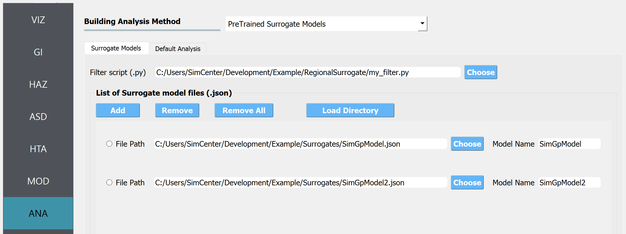
Refer to Step 1 in the EE-UQ documentation for initial steps. Users must complete the Surrogate Models and Default Analysis tabs to use pre-trained surrogate models.

Fig. 2.7.1.5.1 Buildings analysis input panel.

Surrogate Models

• Filter script: A Python script provided by the user to assign surrogate models to buildings when multiple surrogate models representing different building types are provided. The script should contain a function named model distributor that processes dictionary inputs for general information (GI) and structural analysis model parameters (SAM), returning the surrogate model name or “Default”. Below is an example of the filter script.

  
  def model_distributor(GI,SAM):
  
  
  	if GI["NumberOfStories"]==1 and GI["StructureType"]=="W1":
  		modelName ="SimGpModel"
  	elif GI["NumberOfStories"]==2 and GI["StructureType"]=="W1":
  		modelName ="SimGpModel2"
  	else:
  		modelName ="Default"
  	return modelName
  	
  

  Below are example keys and values of GI and SAM dictionaries that will be provided to the model.

  GISAM (MDOF-Lu)

  {
      "AIM_id": "1",
      "location": {
        "latitude": 61.21700019,
        "longitude": -149.9083196
      },
      "Latitude": 61.21700019,
      "Longitude": -149.9083196,
      "NumberOfStories": 2,
      "YearBuilt": 1983,
      "OccupancyClass": "RES1",
      "PlanArea": 3059,
      "StructureType": "W1",
      "units": {
        "force": "kips",
        "length": "ft",
        "time": "sec"
      }
    }
  

• Surrogate models: surrogate model files in JSON (.json) format. Each surrogate model can be separately trained and exported in JSON format through EE-UQ. The surrogate models will take structural parameters (structure information and structural analysis parameters computed in the modeling app (specified in the MOD tab)), and ground motion intensity parameters as inputs. Below, we list the names of the parameters that will be passed to the surrogate model and its example values. When training a surrogate model through EE-UQ, make sure it only expects a subset of the structural variables listed below as inputs (The ground motion parameters are processed automatically internally, so users do not need to be concerned about naming rules on those variables).

  1. Structure information - user-provided inventory data

     Table 2.7.1.5.1 User-provided structure information

     Variable Name	Type	Example Value	Note
     Latitude	double	61.21700019
     Longitude	double	-149.9083196
     NumberOfStories	int	2
     YearBuilt	int	1983
     OccupancyClass	string	RES1
     StructureType	string	W1
     PlanArea	double	3059

  2. Structural properties - variables from the modeling (MOD) application (example for a 2-story building using MDOF-LU)

     Table 2.7.1.5.2 Structural parameters estimated by structural modeling app (specified in the MOD tab)

     Variable Name	Type	Example Value	Note
     K0-1	double	61532397.05	initial stiffness of 1st story
     K0-2	double	61532397.05	initial stiffness of 2nd story
     Sy-1	double	2110124.685	yield strength of 1st story
     Sy-2	double	1406749.79	yield strength of 2nd story
     beta-1	double	1	ultimate deformation of 1st story
     beta-2	double	1	ultimate deformation of 2nd story
     eta-1	double	0.0870354	post-yield stiffness ratio of 1st story
     eta-2	double	0.0870354	post-yield stiffness ratio of 2nd story
     a_k-1	double	0.1	parameter related to unloading stiffness* (1st story)
     a_k-2	double	0.1	parameter related to unloading stiffness* (2nd story)
     gamma-1	double	0.8	pinching factor (1st story)
     gamma-2	double	0.8	pinching factor (2nd story)
     alpha-1	double	3	overstrength factor (1st story)
     alpha-2	double	3	overstrength factor (2st story)
     mass-2	double	284190.3994	mass at 2nd floor
     mass-3	double	284190.3994	mass at 3rd floor
     dampingRatio	double	0.099563339	damping ratio

Refer to MDOF-LU Building Model for more details. Custom modeling apps should follow the specified format for “SAM.json”. See here for an example of SAM.json file.

3. Ground motion parameters (automatically named internally both in EE-UQ and R2D)

   Table 2.7.1.5.3 Ground motion parameters

   Variable Name	Type	Example Value	Note
   eventID	string	site_8040x00001	Name of earthquake time history
   1-PSA(0.5s)-0-1	double	12.0041496	Peak spectral acceleration for 0.5 second, horizontal direction 1
   1-DS575-0-1	double	8.915	Strong motion Duration, horizontal direction 1
   1-SaRatio-0-1	double	0.95366258	Spectral acceleration (Sa) ratio at some user-specified Sa values, horizontal direction 1
   1-PSA(0.5s)-0-2	double	10.13654727	Peak spectral acceleration for 0.5 second, horizontal direction 2
   1-DS575-0-2	double	9.4	Strong motion Duration, horizontal direction 2
   1-SaRatio-0-2	double	0.822609112	Spectral acceleration (Sa) ratio at some user-specified Sa values, horizontal direction 2

R2D ensures only the intensity measures specified during the training of the surrogate model are computed and utilized.

Default Analysis

Choose the analysis engine for cases where the filter script returns “Default”.

2.7.2. Transportation Infrastructure Analysis

2.7.2.1. IMasEDP Analysis Model

Similar to buildings, the IMasEDP application for transportation infrastructure uses the hazard intensity measure (IM) directly as the engineering demand parameter (EDP), bypassing structural analysis.