4.9. E10 - Site Response Analysis

Download files

Download

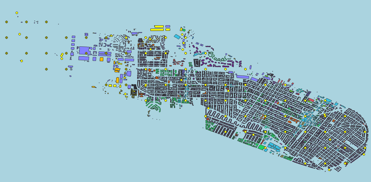
This example presents regional earthquake impact analysis including site response analysis and building damage and loss assessment. Overall 177 sites are included for soil response simulation under bedrock ground motion input with a building inventory including approximately 14,000 buildings in the city of Alameda, CA.

1. Set the Units in the GI panel as shown in Fig. 4.8.1 and check interested output files.

   

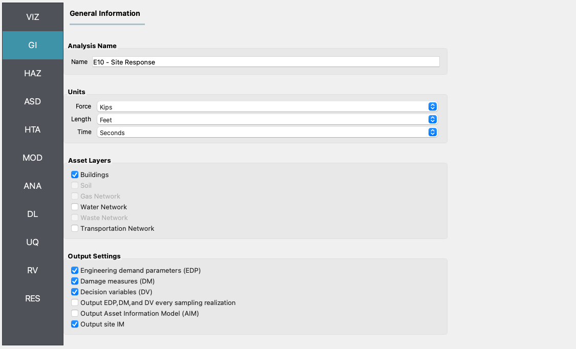
   Fig. 4.9.1 R2D GI setup.

2. Select the Regional Site Response method in the HAZ panel. In the Site input widget, the SiteModelData.csv should be automatically loaded, which includes the basic site information and modelng parameter. In the Soil Properties/Site Response Script widget, the modeling script should be automatically loaded which would create OpenSees tcl models for individual sites selected for analysis. In the Input Motions widget, the EventGrid.csv file as well as the input motion directory should be automatically loaded, which includes the ground acceleration time history data files. In the Units of Event Input File widget, the time history file TH_file has a unit of gravity acceleration and the scaling factor is unitless (these two fields are automatically created from the column headers in EventGrid.csv).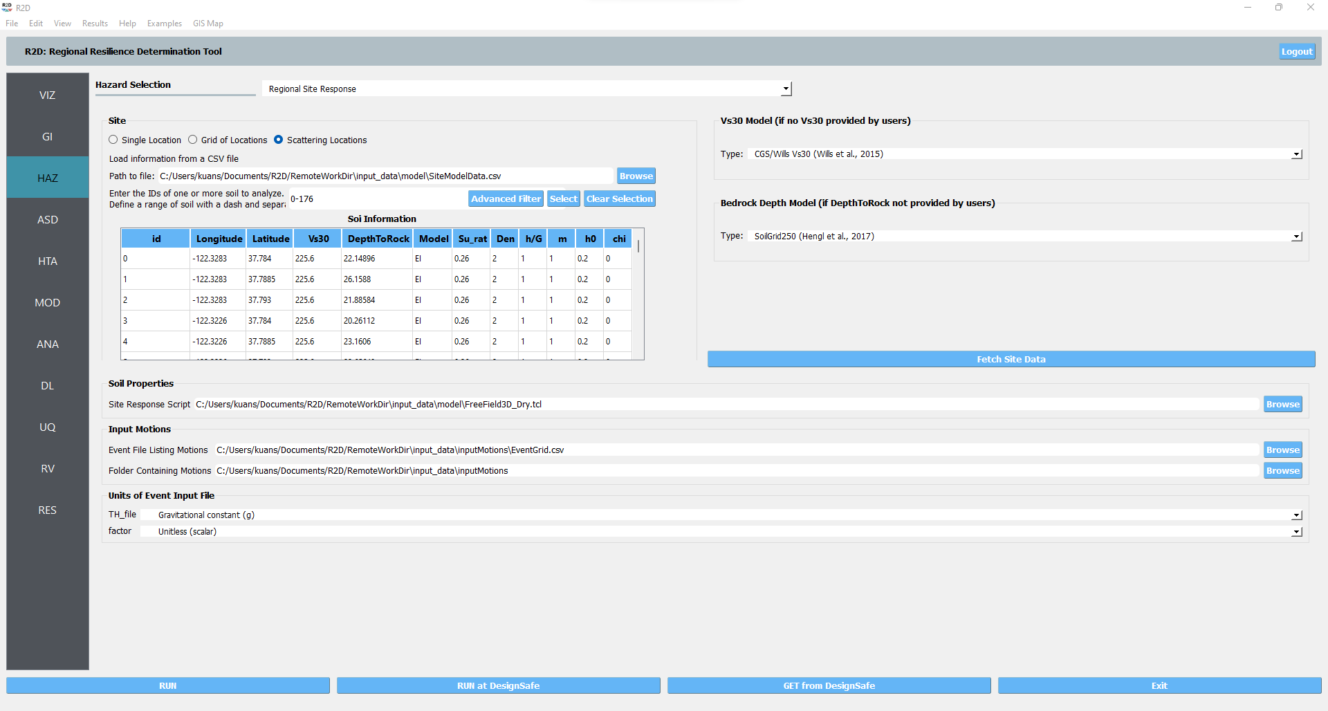

   

   Fig. 4.9.2 R2D HAZ setup.

3. ASD In the asset definition panel, the path to the all_bldgs.csv file is specified. Once this file is loaded, the user can select which particular assets will be included in the analysis by entering a valid range in the form and clicking Select.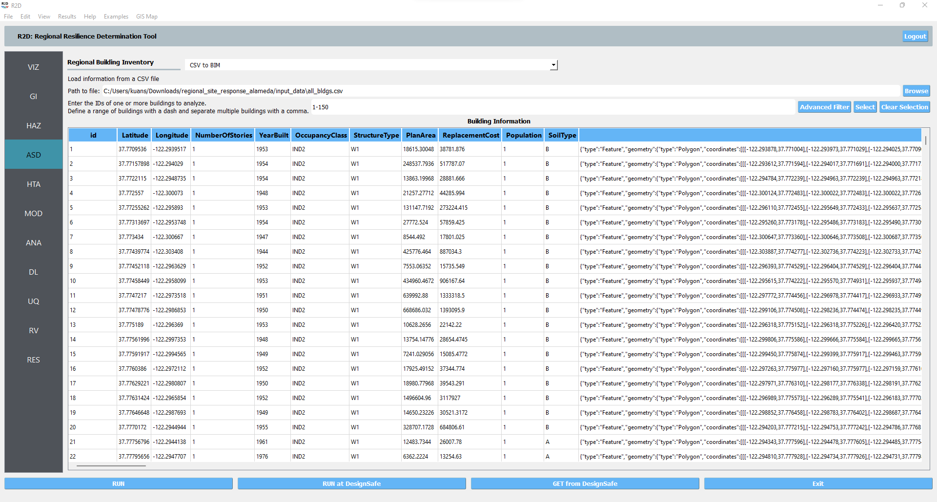

   

   Fig. 4.9.3 R2D ASD setup.

4. HTA Next, a hazard mapping algorithm is specified using the Nearest Neighbor method, which is configured as shown in the following figure with 4 samples in 4 neighbors.

   

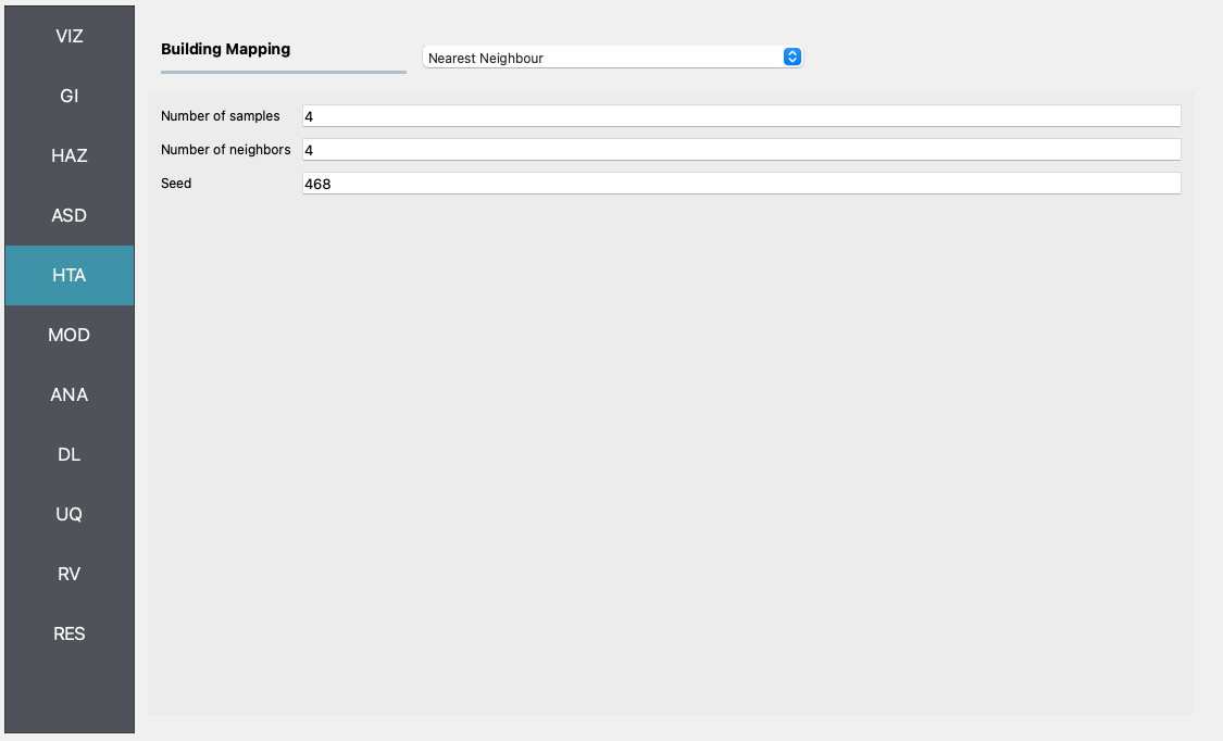
   Fig. 4.9.4 R2D HTA setup.

5. MOD In the modeling panel, the MDOF-LU method is used to create Multi-Degree-Of-Freedom (MDOF) nonlinear shear building model from the input building file in ASD. Following the HAZUS EQ Technical Manual Chapter 5, a hysteretic nonlinear material is defined for each story with a story shear and displacement relationship with the initial stiffness, over-strength ratio, hardening ratio, and degradation factor. These parameters are stored in the HazusData.txt for different building design levels (e.g., high-, moderate-, or pre-code) which is now primarily based on the built year of the structure.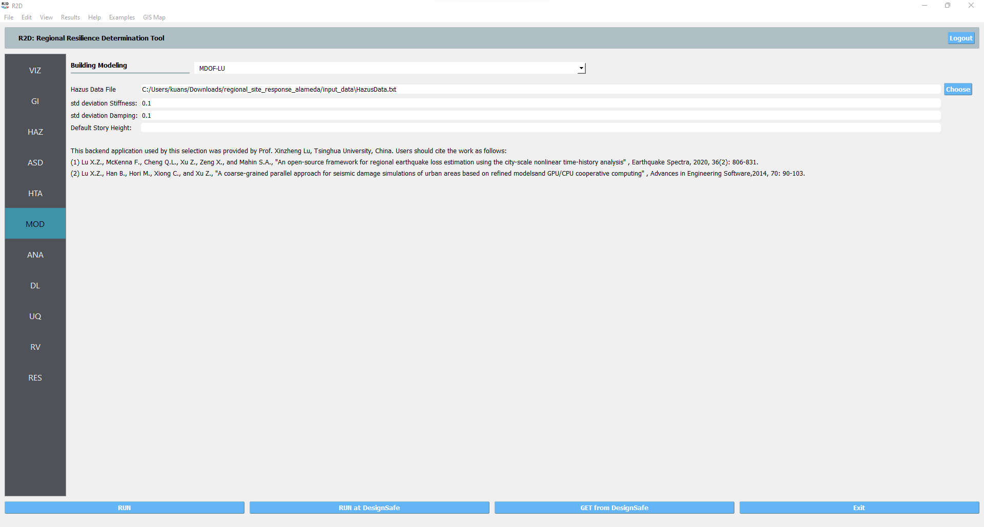

   

   Fig. 4.9.5 R2D MOD setup.

6. Set the “Building Analysis Engine” in ANA panel to “OpenSees”.

   

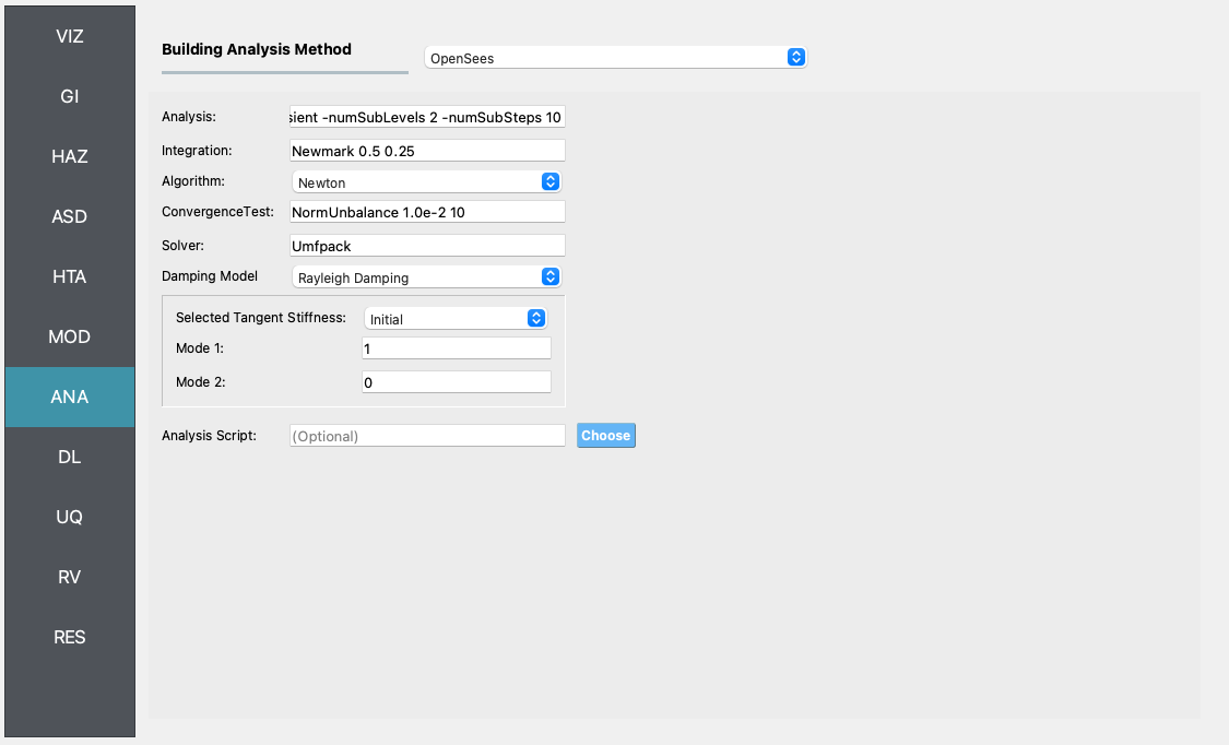
   Fig. 4.9.6 R2D ANA setup.

7. DL The damage and loss panel is now used to configure the Pelicun3 backend. The HAZUS MH EQ Story damage and loss method is selected and configured as shown in the following figure:

   

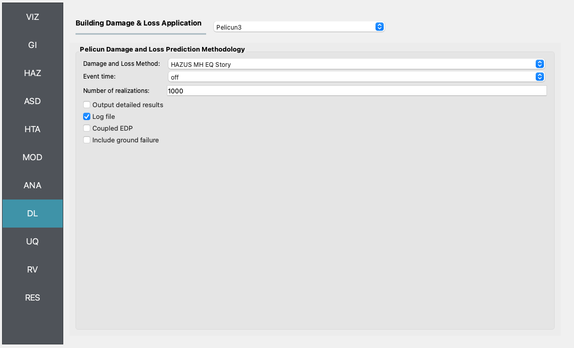
   Fig. 4.9.7 R2D DL setup.

8. Set the “UQ Application” in UQ panel to “Dakota”.

   

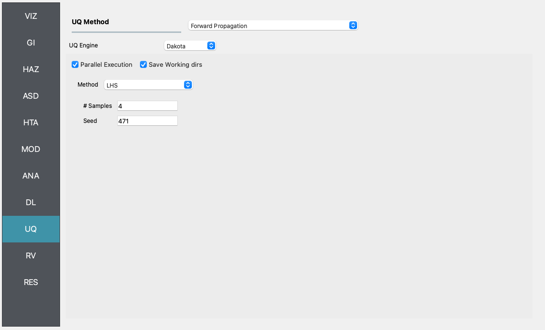
   Fig. 4.9.8 R2D UQ setup.

After setting up the simulation, please click the RUN to execute the analysis. Once the simulation completed, the app would direct you to the RES panel (Fig. 4.8.9) where you could examine and export the results.

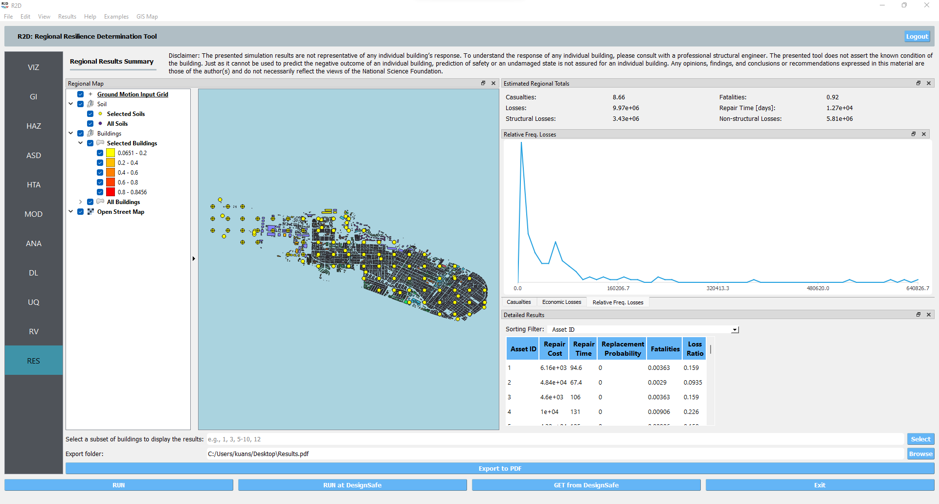
Fig. 4.9.9 R2D RES panel.

For simulating the damage and loss for a large region of interest (please remember to reset the building IDs in ASD), it would be efficient to submit and run the job to DesignSafe on on Frontera. This can be done in R2D by clicking RUN at DesignSafe (one would need to have a valid DesignSafe account for login and access the computing resource). Fig. 4.8.10 provides an example configuration to run the analysis (and please see R2D User Guide for detailed descriptions). The individual site response analysis and building damage and loss simulation are paralleled on Stampede2. It is suggested for this demoed example to use 60 minutes with 96 Skylake (SKX) cores (e.g., 2 nodes with 48 processors per node) to complete the simulation. One would receive a job failure message if the specified CPU hours are not sufficient to complete the run. Note that the product of node number, processor number per node, and buildings per task should be greater than the total number of sites/buildings in the inventory to be analyzed.

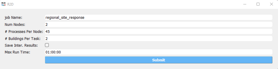
Fig. 4.9.10 R2D - Run at DesignSafe (configuration).

Users could monitor the job status and retrieve result data by GET from DesignSafe button (Fig. 4.8.11). The retrieved data include four major result files, i.e., IM.hdf, BIM.hdf, EDP.hdf, DM.hdf, and DV.hdf. R2D also automatically converts the hdf files to csv files that are easier to work with. While R2D provides basic visualization functionalities (Fig. 4.8.9), users could access the data which are downloaded under the remote work directory, e.g., /Documents/R2D/RemoteWorkDir (this directory is machine specific and can be found in File->Preferences->Remote Jobs Directory). Once having these result files, users could extract and process interested information - the next section will use the results from this testbed as an example to discuss more details.